Lecture 12 Poisson distribution

We have seen three important families of discrete random variables: the Bernoulli, binomial, and geometric distributions. We now look at our fourth and final discrete distribution: the Poisson distribution.

12.1 Definition and properties

Another important distribution is the Poisson distribution. The Poisson distribution (roughly “pwa-song”) is typically used to model “the number of times something happens in a set period of time”. For example, the number of emails you receive in a day; the number of claims at an insurance company each year; or the number of calls to call centre in one hour. (Famously, one of the first historical datasets modelled using a Poisson distribution was “the number of Prussian soldiers in different cavalry units kicked to death by their own horse between 1875 and 1894”.) We’ll explain why the Poisson distribution is a good model for this in the next subsection.

Definition 12.1 Let \(X\) be a discrete random variable with range \(\{0,1,2,\dots\}\) and PMF \[ p_X(x) = \mathrm e^{-\lambda} \frac{\lambda^x}{x!} . \] Then we say that \(X\) follows the Poisson distribution with rate \(\lambda\), and write \(X \sim \text{Po}(\lambda)\).

Here, \(\lambda\) is a lower-case Greek letter “lambda”. I should also note that we interpret \(0! = 1\).

The Poisson distribution is named after the French mathematician Siméon-Denis Poisson who wrote about it in 1837, although the origin of the idea is more than 100 years earlier with another French mathematician, Abraham de Moivre.

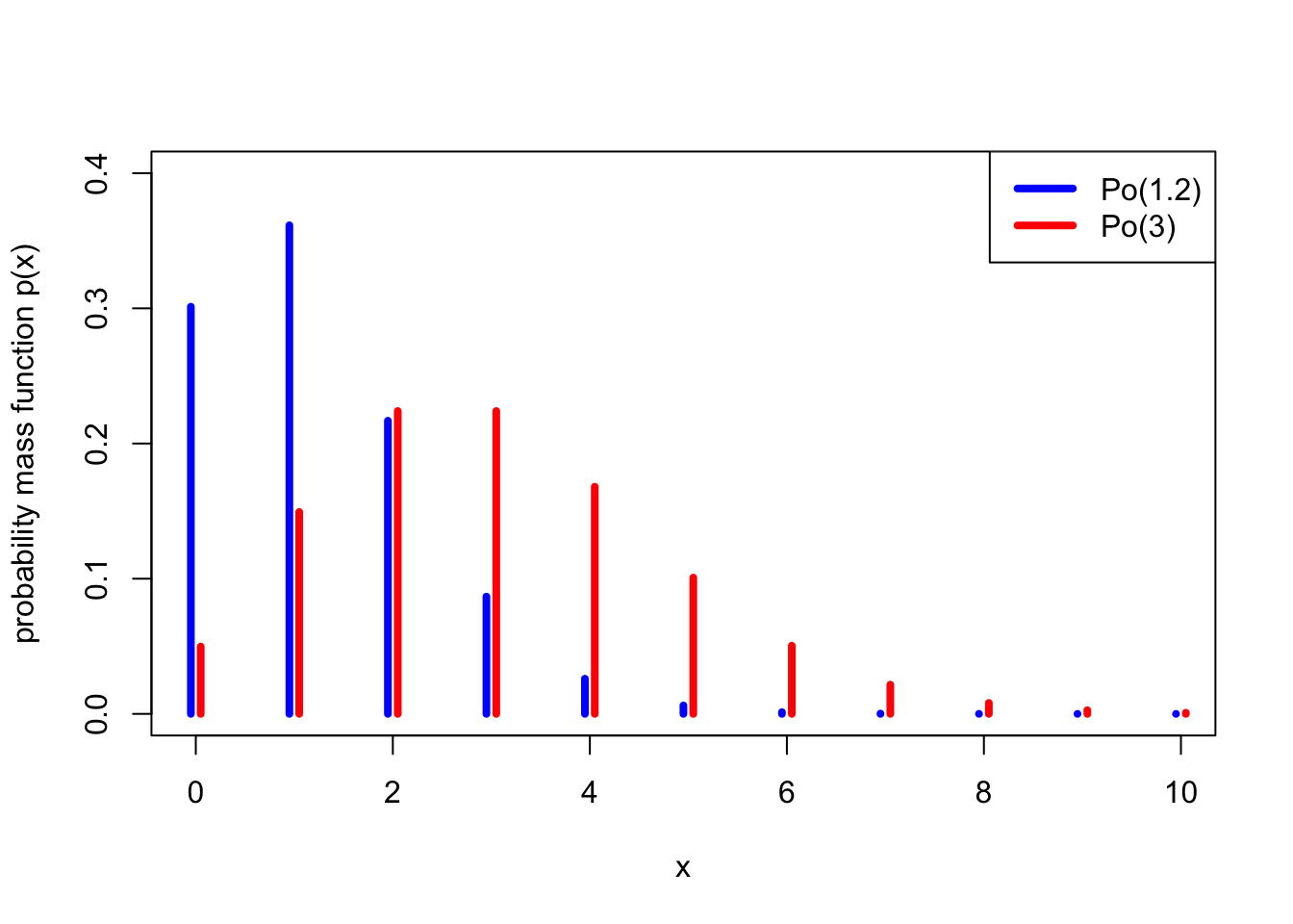
Example 12.1 I receive emails from students at the rate of \(\lambda = 3\) per hour, modelled as a Poisson distribution. What is the probability I get (a) two emails in an hour, (b) no emails in an hour?

The number of emails per hour is \(X \sim \mathrm{Po}(3)\).

For (a), we have \[ \mathbb P(X = 2) = p(2) = \mathrm{e}^{-3} \frac{3^2}{2!} = \frac92 \mathrm{e}^{-3} = 0.224 . \]

For part (b), and remembering that \(0! = 1\), we have \[ \mathbb P(X = 0) = p(0) = \mathrm{e}^{-3} \frac{3^0}{0!} = \mathrm{e}^{-3} = 0.050 . \]

The parameter \(\lambda\) is called the “rate” because that indeed the number of emails (or insurance claims, or phone calls, or deaths by horse-kicking) that we expect to see.

Theorem 12.1 Let \(X \sim \text{Po}(\lambda)\). Then

1. \(p(x)\) is indeed a PMF, in that \(\displaystyle\sum_{x=0}^\infty p(x) = 1\).
2. \(\mathbb EX = \lambda\),
3. \(\operatorname{Var}(X) = \lambda\).

Proof. We’ll do the first two here, then you can do the variance in Problem Sheet 4.

It will be useful to remember the Taylor series for the exponential function, \[ \mathrm e^\lambda = \sum_{x=0}^\infty \frac{\lambda^k}{x!} . \]

For part 1, to see that the PMF does indeed sum to one, note that the Taylor series gives us \[ \sum_{x=0}^\infty p(x) = \sum_{x=0}^\infty \mathrm e^{-\lambda} \frac{\lambda^x}{x!} = \mathrm e^{-\lambda} \sum_{x=0}^\infty \frac{\lambda^x}{x!} = \mathrm e^{-\lambda}\,\mathrm e^{\lambda} = 1. \]

For part 2, for the expectation, we have \[\begin{align*} \mathbb EX &= \sum_{x=0}^\infty x\,\mathrm e^{-\lambda} \frac{\lambda^x}{x!} \\ &= \mathrm e^{-\lambda} \sum_{x=1}^\infty x\,\frac{\lambda^x}{x!} \\ &= \mathrm e^{-\lambda} \sum_{x=1}^\infty \frac{\lambda^x}{(x-1)!} \\ &= \lambda \mathrm e^{-\lambda} \sum_{x=1}^\infty \frac{\lambda^{x-1}}{(x-1)!} \end{align*}\] In the second line, we took \(\mathrm e^{-\lambda}\) outside the sum, and allowed ourselves to start the sum from 1, since the \(x = 0\) term was 0 anyway; in the third line, we cancelled the \(x\) from the \(x!\) to get \((x-1)!\); and in the fourth line we took one of the \(\lambda\)s in \(\lambda^x\) outside the sum, to give ourselves terms in \(x - 1\) inside the sum. We can now “re-index” the sum by putting \(y = x - 1\), to get \[ \mathbb EX = \lambda \mathrm e^{-\lambda} \sum_{y=0}^\infty \frac{\lambda^{y}}{y!} = \lambda \mathrm e^{-\lambda} \mathrm e^{\lambda} = \lambda , \] where we used the Taylor series again.

12.2 Poisson approximation to the binomial

Suppose I own a watch shop in Leeds. My watches are very expensive, so I don’t need to sell many each day – in fact, I sell an average of 4.8 watches per day. How should I model the number of watches sold each day as a random variable?

One way could be to say this. There are \(n\) people living in Leeds and the surrounding area. On any given day, each of those \(n\) people will independently buy a watch from my shop with some probability \(p\). Thus the total number of watches I sell could be modelled as a binomial distribution \(\text{Bin}(n, p)\).

But what should \(n\) and \(p\) be? To make the average \(\mathbb EX = np = 4.8\), I must take \(p = 4.8/n\). But what about \(n\)? We know \(n\) is a very big number, because Leeds is a big city – so let’s take a limit as \(n \to \infty\). It turns out, that this distribution \(\text{Bin}(n, 4.8/n)\) becomes a Poisson(4.8) distribution!

Theorem 12.2 Fix \(\lambda \geq 0\), and let \(X_n \sim \text{Bin}(n, \lambda/n)\) for all integers \(n \geq \lambda\). Then \(X_n \to \text{Po}(\lambda)\) in distribution as \(n \to \infty\), by which we mean that if \(Y \sim \text{Po}(\lambda)\), then \[ p_{X_n}(x) \to p_Y(x) \qquad \text{for all $x \in \{0, 1, \dots \}$}. \]

A looser way to state the principle of this theorem would be this: When \(n\) is very large and \(p\) very small, in such a way that \(np\) is a small-ish number, then \(\text{Bin}(n,p)\) is well approximated by \(\text{Po}(\lambda)\) where \(\lambda = np\).

This is why a Poisson distribution is a good model for the number of occurrences in a set time period. It applies if there lots of things that could happen (large \(n\)), each one is individually unlikely (small \(p\)), and on average a few of them will actually happen (\(\lambda = np\) small-ish).

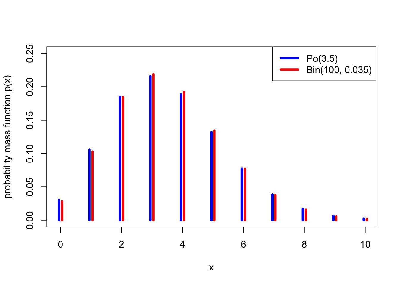
Example 12.2 A lecturer teaches a module with \(n = 100\) students, and estimates that each student turns up to office hours drop-in sessions independently with probability \(p = 0.035\). What is the probability that (a) exactly 5, (b) 2 or more students turn up to a drop-in session?

If we let \(X\) be the number of students that turn up to a drop-in session, then the exact distribution of \(X\) is \(X \sim \text{Bin}(100, 0.035)\).

For part (a), we then have \[ \mathbb P(X = 5) = \binom{100}{5} 0.035^5 (1 - 0.035)^{100-5} = 0.134 . \]

For part (b), we have an “at least” event, so we use the complement rule to get \[\begin{align*} \mathbb P(X \geq 2) &= 1 - \mathbb P(X = 0) - \mathbb P(X = 1) \\ &= 1 - \binom{100}{0} 0.035^0 (1 - 0.035)^{100-0} + \binom{100}{1} 0.035^1 (1 - 0.035)^{100 - 1} \\ &= 1 - (1 - 0.035)^{100} + 100 \times 0.035 (1 - 0.035)^{99} \\ &= 1 - 0.028 - 0.103 \\ &= 0.869 \end{align*}\]

Alternatively, it might be more convenient to approximate \(X\) by a Poisson distribution \(Y \sim \text{Po}(100 \times 0.035) = \text{Po}(3.5)\).

For part (a), this gives \[ \mathbb P(Y = 5) = \mathrm e^{-3.5} \frac{3.5^5}{5!} = 0.132 , \] which is very close to the exact answer above of \(0.134\).

For part (b), the approximation gives \[\begin{align*} \mathbb P(Y \geq 2) &= 1 - \mathbb P(Y = 0) - \mathbb P(Y = 1) \\ &= 1 - \mathrm e^{-3.5} \frac{3.5^0}{0!} - \mathrm e^{-3.5} \frac{3.5^1}{1!} \\ &= 1 - \mathrm e^{-3.5} - 3.5 \mathrm e^{-3.5} \\ &= 1 - 0.030 - 0.106 \\ &= 0.864 \end{align*}\] which is very close to the exact answer above of \(0.869\).

The following graph shows how close the \(\text{Po}(3.5)\) distribution is to a \(\text{Bin}(100, 0.035)\) distribution – not exact, but pretty good.

For completeness, we include a proof of Theorem 12.2 here, although since it discusses use of limits, it’s not examinable material for this module.

Proof. (Non-examinable) We need to show that, as \(n \to \infty\), \[ p_X(x) = \binom nx \left(\frac{\lambda}{n}\right)^x \left(1 - \frac{\lambda}{n}\right)^{n-x} \to \mathrm{e}^{-\lambda} \frac{\lambda^x}{x!} = p_Y(x) . \] Let’s try. The left-hand side is, by some simple rearrangements, \[\begin{align*} \binom nx &\left(\frac{\lambda}{n}\right)^x \left(1 - \frac{\lambda}{n}\right)^{n-x} \\ &= \frac{n(n-1)\cdots(n-x+1)}{x!} \frac{\lambda^x}{n^x} \left(1 - \frac{\lambda}{n}\right)^{n}\left(1 - \frac{\lambda}{n}\right)^{-x} \\ &= \frac{\lambda^x}{x!} \frac{n(n-1)\cdots(n-x+1)}{n^x} \left(1 - \frac{\lambda}{n}\right)^{n}\left(1 - \frac{\lambda}{n}\right)^{-x} \\ &= \frac{\lambda^x}{x!} \frac{n}{n} \frac{n-1}{n} \cdots \frac{n-x+1}{n} \left(1 - \frac{\lambda}{n}\right)^{n}\left(1 - \frac{\lambda}{n}\right)^{-x} \\ &= \frac{\lambda^x}{x!} 1 \left(1 - \frac{1}{n}\right) \cdots \left(1 - \frac{x-1}{n}\right) \left(1 - \frac{\lambda}{n}\right)^{n}\left(1 - \frac{\lambda}{n}\right)^{-x} . \end{align*}\]

Now let’s take each of the terms in turn. First \(\lambda^x / x!\) looks very promising, and can stay. Second, each of the terms \(1, 1 - 1/n, \dots, 1 - (x-1)/n\) tend to 1 as \(n \to \infty\). Third, \[ \left(1 - \frac{\lambda}{n}\right)^{n} \to \mathrm{e}^{-\lambda} ; \] this is from the standard “compound interest” result that \[ \left(1 + \frac{a}{n}\right)^{n} \to \mathrm{e}^{a} \qquad \text{as $n \to \infty$}. \] Finally \[\left(1 - \frac{\lambda}{n}\right)^{-x} \to 1 , \] as \(1 - \lambda/n \to 1\), and \(x\) is fixed. Putting all that together gives the result.

12.3 Distributions as models for data

Families of distributions – like the Bernoulli, binomial, geometric and Poisson distributions we have seen so far in this module – are very useful for models in statistics. The idea of using families of distributions as models for data will be developed in the topic of Bayesian statistics we will discuss in Lectures 19 and 20 of this module, and, even more so, will be extremely important throughout the whole of MATH1712 Probability and Statistics II.

The families of distributions we have looked at here are sometimes called “parametric families”, in that each of the distributions depended on one or more parameters: \(p\) for the Bernoulli and geometric distributions, both \(n\) and \(p\) for the binomial distribution, and \(\lambda\) for the Poisson distribution. (Later in the module we will also see some continuous parametric families: the exponential, normal and beta distributions.) This means we can adopt a model that data comes from one of the distributions within a family, then use data to estimate the value of that parameter.

For example:

• When testing the bias of a coin, you might assume, counting Heads as 1 and Tails as 0, that the outcome of each test is Bernoulli distributed with parameter \(p\), but where the value of the Heads probability \(p\) is unknown. You could then toss the coin many times and use this data to estimate \(p\).

• The number of years between severe summer floods in a tropical climate could be modelled as geometrically distributed where the flood risk parameter \(p\) is unknown. By look at the gaps between severe floods in historical data, a statistician could try to estimate \(p\).

• A tutor might assume that the number of students that turn up to each tutorial is binomially distributed where \(n\) is known to equal 12, the number of students assigned to the group, but \(p\), the “turning-up probability” is unknown. The tutor could then take records of how many students turned up to all the tutorials, and use this to estimate \(p\).

• The number of calls received each day by call centre might be modelled as a Poisson distribution where the rate \(\lambda\) is unknown. The company could exam its records to estimate \(\lambda\).

There are two main methods statisticians use to estimate parameters:

• Bayesian statistics: Here, one starts with a subjective “prior” distribution for the parameters, which represents one’s personal belief about which possible values for that parameter are more or less likely before conducting any experiment. After the experiment, one then uses Bayes’ theorem to update that belief to a “posterior” distribution of one’s beliefs about the parameter given the data. The Bayesian approach will be introduced in Lecture 19 of this module.

• Frequentist statistics: Frequentist statistics does not involve any subjective prior views. Rather, frequentism is about assessing the extent to which the data is consistent with certain hypotheses.

  • You might try to find the value for the parameter that seems “most consistent” with the data, and use that as an estimate of the parameter: “My best guess of the Heads probability \(p\) of the coin is \(p = 0.53\).
  • You might find a range of values for the parameter that are all at least somewhat consistent with the data: “I am confident the value of the Heads probability lies in the range \(0.49 \leq p \leq 0.57\), as these values are all consistent with the data.”
  • You could test if a specific hypothesis is consistent with the data or not: “The data is consistent with the hypothesis that \(p = 0.50\), which would mean the coin is fair, so I have no strong evidence for concluding that the coin is biased.”

The frequentist approach will pursued in detail throughout MATH1712.

Summary

Distribution	Range	PMF	Expectation	Variance
Bernoulli: \(\text{Bern}(p)\)	\(\{0,1\}\)	\(p(0) = 1- p\), \(p(1) = p\)	\(p\)	\(p(1-p)\)
Binomial: \(\text{Bin}(n,p)\)	\(\{0,1,\dots,n\}\)	\(\displaystyle\binom{n}{x} p^x (1-p)^{n-x}\)	\(np\)	\(np(1-p)\)
Geometric: \(\text{Geom}(p)\)	\(\{1,2,\dots\}\)	\((1-p)^{x-1}p\)	\(\displaystyle\frac{1}{p}\)	\(\displaystyle\frac{1-p}{p^2}\)
Poisson: \(\text{Po}(\lambda)\)	\(\{0,1,\dots\}\)	\(\mathrm{e}^{-\lambda} \displaystyle\frac{\lambda^x}{x!}\)	\(\lambda\)	\(\lambda\)

• Stirzaker, Elementary Probability, Section 4.2.
• Grimmett and Welsh, Probability, Section 2.2.