Lecture 19 Bayesian statistics I

In this final section of the module, we return to statistics, where we will look at an approach to data analysis known as “Bayesian statistics”.

Statistics concerns how to draw conclusions from data; and Bayesian statistics is one particular framework for doing this. The idea of Bayesian statistics is that we start with “prior” (“before”) beliefs about the underlying model, then use the data (together with Bayes’ theorem) to update our to our “posterior” (“after”) beliefs about the model given the data we have observed.

19.1 Example: fake coin?

We will start by illustrating the main idea with an example.

Example 19.1 A joke shop sells three types of coins: normal fair coins; Heads-biased coins, which land Heads with probability 0.8; and Tails-biased coins, which land Heads with probability 0.2. I pick up a coin and examine it; since it looks mostly like a normal coin, I believe there’s 60% chance it’s s fair coin, and a 20% chance it’s biased either way. I decide to toss the coin three times, to gather some more evidence. The result is that all three are Heads. How should I update my beliefs?

So, we start with the “prior” (before) belief \[ \mathbb P(\text{fair}) = 0.6 \qquad \mathbb P(\text{H-bias}) = 0.2 \qquad \mathbb P(\text{T-bias}) = 0.2 \]

We know how to update our beliefs after seeing the data: we use Bayes’ theorem. We have \[\begin{align*} \mathbb P(\text{fair} \mid \text{HHH}) &= \frac{\mathbb P(\text{fair})\, \mathbb P(\text{HHH}\mid \text{fair})}{\mathbb P(\text{HHH})} = \frac{0.6 \times 0.5^3}{\mathbb P(\text{HHH})} = \frac{0.075}{\mathbb P(\text{HHH})} \\ \mathbb P(\text{H-bias} \mid \text{HHH}) &= \frac{\mathbb P(\text{H-bias})\, \mathbb P(\text{HHH}\mid \text{H-bias})}{\mathbb P(\text{HHH})} = \frac{0.2 \times 0.8^3}{\mathbb P(\text{HHH})} = \frac{0.1024}{\mathbb P(\text{HHH})} \\ \mathbb P(\text{T-bias} \mid \text{HHH}) &= \frac{\mathbb P(\text{H-bias})\, \mathbb P(\text{HHH}\mid \text{T-bias})}{\mathbb P(\text{HHH})} = \frac{0.2 \times 0.2^3}{\mathbb P(\text{HHH})} = \frac{0.0016}{\mathbb P(\text{HHH})} . \end{align*}\] We also need to find common denominator \(\mathbb P(\text{HHH})\). We could do that using the law of total probability. But a convenient short-cut is to notice that the above three probabilities have to add up to 1, and so that common denominator must be $0.075 + 0.1024 + 0.0016 = 0.179, so we have \[\begin{align*} \mathbb P(\text{fair} \mid \text{data}) &= \frac{0.075}{0.179} = 0.419 \\ \mathbb P(\text{H-bias}\mid \text{data}) &= \frac{0.1024}{0.179} = 0.572 \\ \mathbb P(\text{T-bias}\mid \text{data}) &= \frac{0.0016}{0.179} = 0.009 . \end{align*}\]

So, after tossing the coin three times, our belief has been updated from the “prior” (before) belief \[ \mathbb P(\text{fair}) = 0.6 \qquad \mathbb P(\text{H-bias}) = 0.2 \qquad \mathbb P(\text{T-bias}) = 0.2 \] to the “posterior” (after) belief \[ \mathbb P(\text{fair} \mid \text{data}) = 0.419 \qquad \mathbb P(\text{H-bias}\mid \text{data}) = 0.572 \qquad \mathbb P(\text{T-bias}\mid \text{data}) = 0.009 . \] Compared to our prior beliefs, our belief that the coin is fair has decreased a little bit; our belief the coin is biased towards Heads has shot up, and is now our most likely belief; while our belief the coin is biased towards Tails has plummeted to just 1%.

19.2 Bayesian framework

Let’s think more systematically about what we did in the previous example.

• Model: The three coin tosses were modelled as three IID Bernoulli trials \(X_1, X_2, X_3 \sim \text{Bern}(\theta)\) (if we let \(X_i = 1\) denote that the \(i\)th coin was Heads). Here, the probability of Heads is some unknown parameter \(\theta\). (Recall we talked about parametric models for data in Subsection 12.3.) This model gives a distribution that depends on the parameter. Here we had a conditional PMF for one trial \[ p(x \mid \theta) = \theta^{x} (1 - \theta)^{1- x} \] (this is a convenient way of writing the PMF for a Bernoulli trial). So the joint PMF for the IID trials is \[ p(\mathbf x \mid \theta) = \prod_{i=1}^3 \theta^{x_i} (1 - \theta)^{1- x_i} = \theta^{\sum_i x_i} (1 - \theta)^{3- \sum_i x_i} . \] (Here and throughout, \(\prod\), the Greek capital Pi, means a product – it’s the multiplication equivalent of the summation Sigma, \(\Sigma\).)
• Prior: We started with a prior belief \(\pi(\theta)\) on the value of the unknown parameter. In our case, we had the PMF \[ \pi(0.2) = 0.2 \qquad \pi(0.5) = 0.6 \qquad \pi(0.8) = 0.2 . \]
• Data: We collected the data \(\mathbf x\), which here had \(x_1 = 1\), \(x_2 = 1\), \(x_3 = 1\) (with 1 denoting Heads and 0 denoting Tails).
• Posterior: We calculated the posterior distribution \(\pi(\theta \mid \mathbf x)\) for the parameter given the data. We did this using Bayes’ theorem: \[ \pi(\theta \mid \mathbf x) = \frac{\pi(\theta) \, p(\mathbf x \mid \theta)}{p(\mathbf x)} \propto \pi(\theta) \, p(\mathbf x \mid \theta) .\] We recovered the constant of proportionality – that is, the denominator of Bayes’ theorem – because we knew \(\pi(\theta \mid \mathbf x)\) was a conditional PMF so must add up to 1. We ended up with \[ \pi(0.2 \mid \mathbf x) = 0.009 \qquad \pi(0.5 \mid \mathbf x) = 0.419 \qquad \pi(0.8 \mid \mathbf x) = 0.572 . \]

This is the framework of how Bayesian statistics works: model, prior, data, posterior. To lay it out more generally, the procedure goes like this:

• Model: We start with a model for the data \(\mathbf x\) that depends on one or more parameters \(\theta\), as expressed by a conditional PMF (for discrete data) or PDF (for continuous data) \(p(\mathbf x \mid \theta)\). This normally represents \(n\) IID experiments, so \[ p(\mathbf x \mid \theta) = \prod_{i=1}^n p(x_i \mid \theta) . \] This conditional distribution is often called the likelihood.
• Prior: We have a prior distribution \(\pi(\theta)\) for the parameter \(\theta\), which can be either a PMF or PDF. The prior distribution represents our beliefs about the parameter before we collect the data; this can be based on previous evidence, expert opinion, personal intuition, etc.
• Data: We collect the data \(\mathbf x\).
• Posterior: We then form the posterior distribution \(\pi(\theta \mid \mathbf x)\) for the parameter given the data, using Bayes’ theorem: \[\begin{align*} \pi(\theta \mid \mathbf x) &\propto \pi(\theta)\, p(\mathbf x \mid \theta) \\ \text{posterior} &\propto \text{prior} \times \text{likelihood} . \end{align*}\] This can either be a conditional PMF or PDF, but will be the same type as the prior \(\pi(\theta)\).

19.3 Beta distribution

In our fake-coin example, we had a prior PMF for the parameter \(\theta = p\) that could only take one of three possible values. But when doing Bayesian statistics with a parameter that represents a probability, it makes more sense to have a prior PDF that covers the whole interval \([0,1]\). After all, any parameter value that is given a probability of 0 in the prior always has a probability 0 in the posterior as well, no matter how strong the evidence in its favour; it’s considered good practice to only put 0 prior probability on parameter values that are literally impossible, such as probabilities below 0 or above 1. (This is sometimes called “Cromwell’s rule”.)

One useful family of distributions to use as a prior distribution for a probability parameter is the Beta distribution, whose range is the whole interval \([0,1]\).

Definition 19.1 A continuous random variable \(X\) is said to have the Beta distribution with parameters \(\alpha\) and \(\beta\) if it has the PDF \[ f(x) = \frac{1}{B(\alpha, \beta)} x^{\alpha-1} (1-x)^{\beta - 1} \qquad \text{for $0 \leq x \leq 1$} \] and 0 otherwise. Here, the constant \[ B(\alpha, \beta) = \int_0^1 x^{\alpha-1} (1-x)^{\beta - 1} \, \mathrm dx , \] known as the “Beta function”, ensures that the PDF integrates to 1. We write \(X \sim \text{Beta}(\alpha, \beta)\).

Theorem 19.1 Let \(X \sim \text{Beta}(\alpha,\beta)\). Then

1. \(\mathbb EX = \displaystyle\frac{\alpha}{\alpha + \beta}\)
2. \(\operatorname{Var}(X) = \displaystyle\frac{\alpha\beta}{(\alpha+\beta)^2(\alpha+\beta+1)} = \displaystyle\frac{\mu(1-\mu)}{\alpha+\beta + 1}\), where \(\mu = \mathbb EX\).

(Proving this requires some awkward messing around with Gamma functions, which we won’t bother with here.)

So the idea is that the expectation of \(X\) is decided on by the relative values of \(\alpha\) and \(\beta\), while the variance is decided by the total value of \(\alpha\) and \(\beta\). The following two pictures illustrate this:

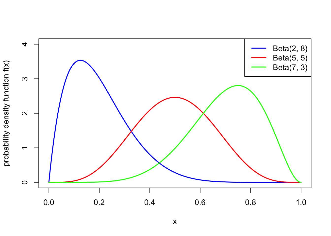
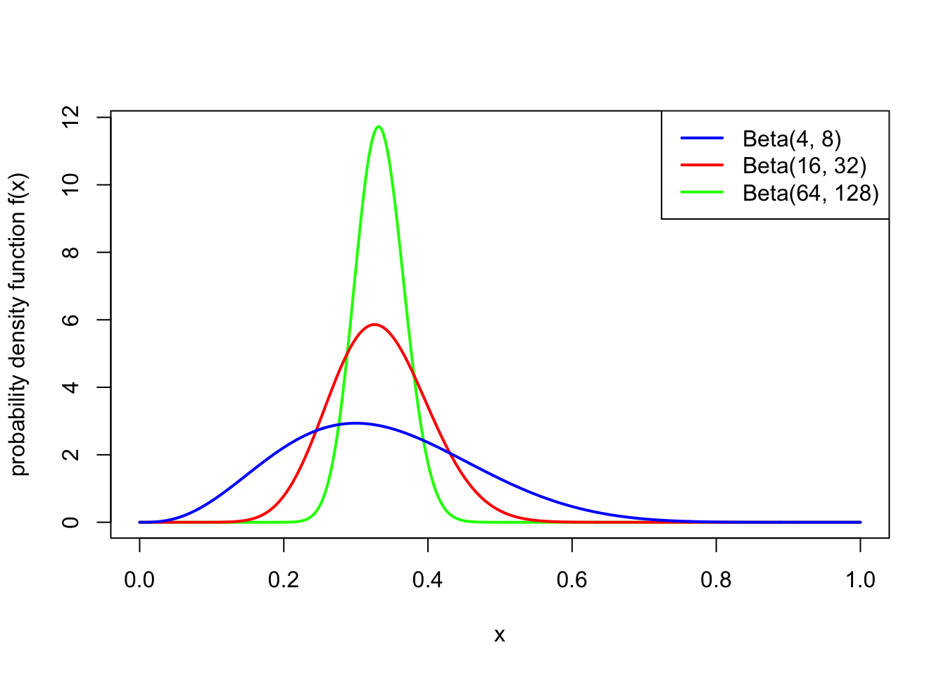
Note also that \(\text{Beta}(1,1)\) is the continuous uniform distribution from Example 15.1.

Example 19.2 A statistician is studying the probability \(\theta\) that ordinary coins land Heads. She would like to use a prior distribution for \(\theta\) with prior expectation \(0.5\) and prior standard deviation \(0.01\). What Beta distribution would be appropriate to use?

To get \(\mathbb E\theta = 0.5\), we need \(\alpha = \beta\). Then the variance, which needs to be \(0.01^2 = 0.0001\), is \[ \operatorname{Var}(\theta) = \frac{\mu(1-\mu)}{\alpha+\beta+1} = \frac{0.25}{\alpha + \beta + 1} . \] This requires \(\alpha = \beta = 1250\). (Well, actually \(1249.5\).)