Lecture 17 Exponential distribution and multiple continuous random variables

This lecture is really two mini-lectures stuck together. In the first mini-lecture, we look at another important continuous distribution, the exponential distribution. In the second mini-lecture, we look at the theory of multiple continuous random variables, and find it’s very similar to what we already know about multiple discrete random variables.

17.1 Exponential distribution

An important continuous distribution is the exponential distribution. The exponential distribution is often used to represent lengths of time: for example, the time until a radioactive particle decays, the time between eruptions of a volcano, or the time you have to wait for a bus to arrive at a bus stop.

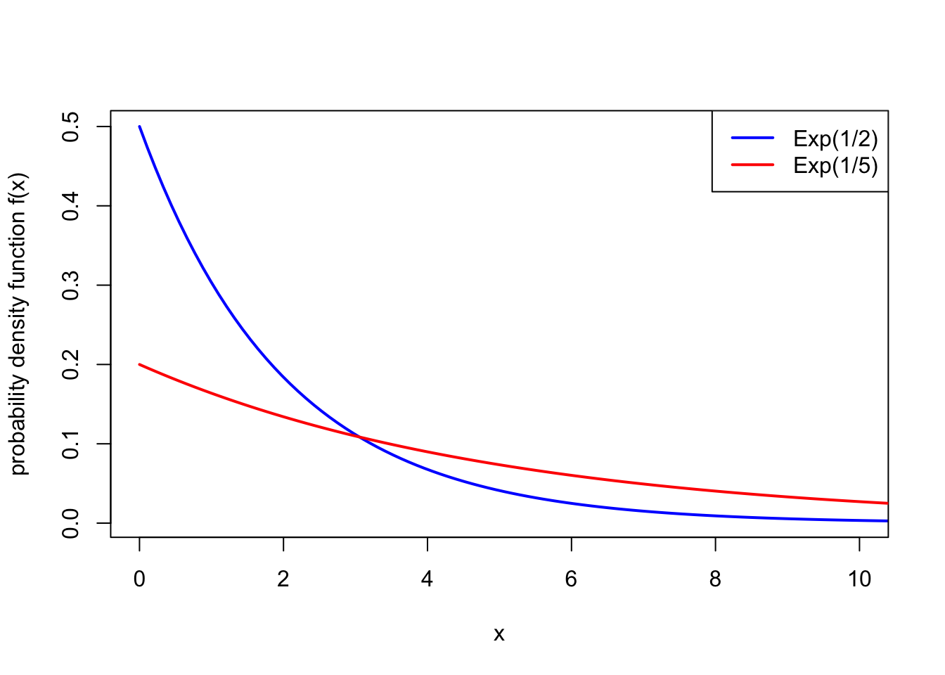
Definition 17.1 A continuous random variable $X$ is said to have the exponential distribution with rate $\lambda > 0$ if it has the PDF \[ f(x) = \lambda \mathrm{e}^{-\lambda x} \qquad \text{for $x \geq 0$}, \] and 0 otherwise. We write $X \sim \text{Exp}(\lambda)$.

Example 17.1 The length of time in years that a lightbulb works before needing to be replaced is modelled as an exponential distribution with rate $\lambda = 2$. What is the probability the lightbulb lasts more than a year but less than three years?

If $X \sim \text{Exp}(2)$ is the lifetime of the lightbulb, we seek $\mathbb P(1 \leq X \leq 3)$. This is \[ \int_{1}^3 f(x)\, \mathrm{d}x = \int_1^3 2 \mathrm e^{-2x} \, \mathrm dx = \big[ -\mathrm e^{-2x} \big]_1^3 = -\mathrm e^{-6} -(-\mathrm e^{-2}) = 0.132. \]

Theorem 17.1 Suppose $X \sim \text{Exp}(\lambda)$. Then:

$f$ is indeed a PDF, in that $\displaystyle\int_0^\infty f(x)\,\mathrm{d}x = 1$;
the CDF of $X$ is $F(x) = 1 - \mathrm{e}^{-\lambda x}$;
the expectation of $X$ is $\mathbb EX = \displaystyle\frac{1}{\lambda}$;
the variance of $X$ is $\operatorname{Var}(X) = \displaystyle\frac{1}{\lambda^2}$.

Example 17.2 Returning to the lightbulb example, where $X \sim \text{Exp}(2)$, we see that the average lifetime of a lightbulb is $\mathbb EX = \frac12$ a year with variance $\operatorname{Var}(X) = \frac14$.

We could alternatively calculate $\mathbb P(1 \leq X \leq 3)$, using the the CDF: \[ \mathbb P(1 \leq X \leq 3) = F(3) - F(1) = (1 - \mathrm{e}^{-2\times 3}) - (1 - \mathrm{e}^{-2\times 1}) = \mathrm{e}^{-2} - \mathrm{e}^{-6} = 0.132 , \] which is the same answer as before.

Proof. of Theorem 17.1. For part 1, \[ \int_0^\infty \lambda \mathrm{e}^{-\lambda x}\,\mathrm{d}x = \big[-\mathrm{e}^{-\lambda x} \big]_0^\infty = -0 -(-1) = 1 . \]

Similarly for part 2, \[ F(x) = \int_0^x \lambda \mathrm{e}^{-\lambda y}\,\mathrm{d}y = \big[-\mathrm{e}^{-\lambda y} \big]_0^x = -\mathrm{e}^{-\lambda x} -(-1) = 1 - \mathrm{e}^{-\lambda x}. \]

For parts 3 and 4, we will use integration by parts, in the form \[ \int_a^b uv' \, \mathrm dx = \big[uv\big]_a^b - \int_a^b u'v \, \mathrm dx , \] where the dash $'$ denotes the derivative.

For part 3, we use integration by parts with $u = x$ and $v' = \lambda \mathrm{e}^{-\lambda x}$, so $u' = 1$ and $v = -\mathrm{e}^{-\lambda x}$. We get \[\begin{align*} \mathbb EX &= \int_0^\infty x \lambda \mathrm{e}^{-\lambda x}\,\mathrm{d}x \\ &= \big[-x \mathrm{e}^{-\lambda x}\big]_0^\infty + \int_0^\infty \mathrm{e}^{-\lambda x}\,\mathrm{d}x \\ &= -0 - (-0) + \left[ -\frac{1}{\lambda} \mathrm{e}^{-\lambda x} \right]_0^\infty \\ &= -0 - \left(- \frac{1}{\lambda}\right) \\ &= \frac{1}{\lambda} \end{align*}\]

For part 4, we will use the computational formula \[ \operatorname{Var}(X) = \mathbb EX^2 - \mu^2 . \] We already know that $\mu = \mathbb EX = 1/\lambda$, so we need $\mathbb EX^2$. We use integration by parts with $u = x^2$ and $v' = \lambda \mathrm{e}^{-\lambda x}$, so $u' = 2x$ and $v = -\mathrm{e}^{-\lambda x}$ again. We get \[\begin{align*} \mathbb EX^2 &= \int_0^\infty x^2 \lambda \mathrm{e}^{-\lambda x}\,\mathrm{d}x \\ &= \big[-x^2 \mathrm{e}^{-\lambda x}\big]_0^\infty + \int_0^\infty 2x \mathrm{e}^{-\lambda x}\,\mathrm{d}x \\ &= -0 - (-0) + \frac{2}{\lambda} \int_0^\infty \lambda x \mathrm{e}^{-\lambda x}\,\mathrm{d}x \\ &= \frac{2}{\lambda} \mathbb EX \\ &= \frac{2}{\lambda^2} , \end{align*}\] where we used a cunning trick on the integral on the right – spotting that we could turn it into the expectation, which is $1/\lambda$, by part 3 – to save us the effort of doing another integration by parts (which would also be a perfectly legitimate way of continuing the proof). Hence \[ \operatorname{Var}(X) = \mathbb EX^2 - \left(\frac{1}{\lambda}\right)^2 = \frac{2}{\lambda^2} - \frac{1}{\lambda^2} = \frac{1}{\lambda^2} . \]

17.2 Multiple continuous random variables

The theory we set up for two or more discrete random variables also works for two or more continuous random variables.

Now, the intensity of probability for $(X,Y)$ being around $(x,y)$ is given by the joint probability density function $f_{X,Y}$. In particular for $a \leq b$ and $c \leq d$, we have that \[ \mathbb P(a \leq X \leq b \text{ and } c \leq Y \leq d ) = \int_{x = a}^b \int_{y = c}^d f_{X,Y}(x,y)\, \mathrm dy \,\mathrm dx \] is given by a double integral.

Discrete random variables	Continuous random variables
We can get the marginal PMF $p_X$ of $X$ by summing over $y$, so \[ p_X(x) = \sum_y p_{X,Y}(x,y) . \]	We can get the marginal PDF $f_X$ of $X$ by integrating over $y$, so \[ f_X(x) = \int_{-\infty}^\infty f_{X,Y}(x,y) \, \mathrm dy. \]
Two discrete random variables $X$ and $Y$ are independent if their PMFs satisfy \[p_{X,Y}(x,y) = p_X(x)\,p_Y(y) \qquad \text{for all $x, y$}.\]	Two continuous random variables $X$ and $Y$ are independent if they have PDFs which satisfy \[f_{X,Y}(x,y) = f_X(x)\,f_Y(y) \qquad \text{for all $x, y$}.\]
The conditional PMF of $Y$ given $X$ is defined by \[ p_{Y \mid X}(y \mid x) = \frac{p_{X,Y}(x,y)}{p_X(x)} . \]	The conditional PDF of $Y$ given $X$ is defined by \[ f_{Y \mid X}(y \mid x) = \frac{f_{X,Y}(x,y)}{f_X(x)} . \]
Bayes’ theorem states that \[ p_{X \mid Y}(x \mid y) = \frac{p_X(x)\,p_{Y\mid X}(y\mid x)}{p_Y(y)} . \]	Bayes’ theorem states that \[ f_{X \mid Y}(x \mid y) = \frac{f_X(x)\,f_{Y\mid X}(y\mid x)}{f_Y(y)} . \]
The expectation of a function of $X$ and $Y$ is given by the sum \[ \mathbb Eg(X,Y) = \sum_{x,y} g(x,y)\, p_{X,Y}(x,y) . \]	The expectation of a function of $X$ and $Y$ is given by the integral \[ \mathbb Eg(X,Y) = \int_{-\infty}^\infty \int_{-\infty}^\infty g(x,y)\, f_{X,Y}(x,y) \, \mathrm dx \, \mathrm dy . \]
The covariance of $X$ and $Y$ is given by \[ \operatorname{Cov}(X,Y) = \mathbb E(X - \mu_X)(Y - \mu_Y) , \] and has a computational formula \[ \operatorname{Cov}(X,Y) = \mathbb EXY - \mu_X \mu_Y . \]	The covariance of $X$ and $Y$ is given by \[ \operatorname{Cov}(X,Y) = \mathbb E(X - \mu_X)(Y - \mu_Y) , \] and has a computational formula \[ \operatorname{Cov}(X,Y) = \mathbb EXY - \mu_X \mu_Y . \]

Example 17.3 Consider the pair of continuous random variables $X$ and $Y$ with joint PDF \[ f_{X,Y}(x,y) = \tfrac45(1 + xy) \qquad \text{for $0 \leq x,y\leq 1$} \] and $f_{X,Y}(x,y) = 0$ otherwise.

First, let’s find the marginal PDF for $X$. We find this by integrating over $y$, so \[\begin{align*} f_X(x) &= \int_{y=-\infty}^\infty f_{X,Y}(x,y) \, \mathrm{d}y \\ &= \int_{y = 0}^1 \tfrac45 (1 + xy) \, \mathrm dy \\ &= \tfrac45 \left[y + \tfrac12 xy^2 \right]_{y=0}^1 \\ &= \tfrac45 \left(1 + \tfrac12x - 0 - 0 \right) \\ &= \tfrac45 \left(1 + \tfrac12x \right) . \end{align*}\] In the second line we, substituted in the joint PDF, and since that is 0 for $y<0$ and $y>1$, we only needed to consider the integral from 0 to 1; in the third line, we integrated with respect to $y$, treating $x$ as a constant; the fourth evaluated the integral, and the fifth line tidied up the answer.

Second, let’s find the conditional PDF for $Y$ given $X = \frac14$. We know that \[ f_{Y\mid X} \big(y \mid \tfrac14\big) = \frac{f_{X, Y} (\tfrac14, y)}{f_X(\frac14)} . \] The numerator is \[ f_{X, Y} \big(\tfrac14, y\big) = \tfrac45 \big(1 + \tfrac14y\big) , \] and the denominator is \[ f_X\big(\tfrac14\big) = \tfrac 45 \big(1 + \tfrac12\times \tfrac 14\big) = \tfrac45 \times \tfrac 98 , \] using the marginal PMF $f_X$ calculated earlier. Hence \[ f_{Y\mid X} \big(y \mid \tfrac14\big) = \frac{\tfrac45 (1 + \tfrac14y)}{\tfrac45 \times \tfrac 98} = \tfrac89 \big(1 + \tfrac14y\big) . \]

Third, let’s find the covariance. We will use the computational formula \[ \operatorname{Cov}(X, Y) = \mathbb EXY - \mu_X \mu_Y . \]

To find $\mu_X = \mathbb EX$, using the marginal PMF $f_x$, we have \[\begin{align*} \mu_X = \mathbb EX &= \int_{-\infty}^{\infty} x\,f(x)\, \mathrm dx \\ &= \int_0^1 x \, \tfrac45 \big(1 + \tfrac12 x\big)\,\mathrm dx \\ &= \tfrac45 \int_0^1 \big(x + \tfrac12 x^2 \big) \, \mathrm dx \\ &= \tfrac45 \left[ \tfrac12x^2 + \tfrac16 x^3 \right]_0^1 \\ &= \tfrac45 \big(\tfrac12 + \tfrac16 - 0 - 0 \big) \\ &= \tfrac{8}{15}. \end{align*}\] (Again, because the PMF is 0 outside the interval from 0 to 1, we can restrict our integral to that.)

To find $\mu_Y = \mathbb EY$, we could go through the process of finding the marginal PDF by integrating over $x$, then calculating $\mu_Y$ as another integral. Alternatively, we could recognise that the joint PMF $f_{X,Y}(x,y) = \frac45 (1+xy)$ is symmetric in $x$ and $y$, so we must have $\mu_Y = \mu_X = \frac{8}{15}$.

We also need $\mathbb EXY$. Using the law of the unconscious statistician, we have \[\begin{align*} \mathbb EXY &= \int_{x = -\infty}^{\infty} \int_{y = -\infty}^{\infty} xy\, f_{X,Y}(x,y)\, \mathrm dy\, \mathrm dx \\ &= \int_{x = 0}^{1} \int_{y = 0}^{1} xy \, \tfrac45 (1+xy) \, \mathrm dy\, \mathrm dx \\ &= \tfrac45 \int_{x = 0}^{1} \int_{y = 0}^{1} (xy + x^2y^2)\, \mathrm dy\, \mathrm dx . \end{align*}\] We’ll do the integral over $y$ first (although either order is fine). This means we integrate treating $x$ as a constant, so we get \[\begin{align*} \mathbb EXY &= \tfrac45 \int_{x = 0}^{1} \int_{y = 0}^{1} (xy + x^2y^2)\, \mathrm dy\, \mathrm dx \\ &= \tfrac45 \int_{x = 0}^{1} \left[ \tfrac12 xy^2 + \tfrac13 x^2y^3 \right]_{y=0}^1 \, \mathrm dx \\ &= \tfrac45 \int_{x = 0}^{1} \big( \tfrac12x + \tfrac13 x^2 - 0 - 0\big) \, \mathrm dx \\ &= \tfrac45 \int_{x = 0}^{1} \big( \tfrac12x + \tfrac13 x^2\big) \, \mathrm dx . \end{align*}\] We then integrate that over $x$, to get \[\begin{align*} \mathbb EXY &= \tfrac45 \int_{x = 0}^{1} \big( \tfrac12x + \tfrac13 x^2\big) \, \mathrm dx \\ &= \tfrac45 \left[ \tfrac14 x^2 + \tfrac19 x^3 \right]_{x=0}^1 \\ &= \tfrac45 \big(\tfrac14 + \tfrac19 - 0 - 0 \big) \\ &= \tfrac{13}{45} \end{align*}\]

Hence, the covariance is \[ \operatorname{Cov}(X, Y) = \mathbb EXY - \mu_X \mu_Y = \tfrac{13}{45} - \tfrac{8}{15} \times \tfrac{8}{15} = \tfrac{1}{255} = 0.0044 , \] which is a slightly positive covariance.

Summary

The exponential distribution has PDF $f(x) = \lambda \mathrm e^{-\lambda x}$, expectation $1/\lambda$, and variance $1/\lambda^2$.
Most properties of multiple discrete random variables carry of to multiple continuous random variables. To get a marginal PDF from a joint PDF, we integrate (rather than sum) over the other variable.

Discrete random variables	Continuous random variables
We can get the marginal PMF \(p_X\) of \(X\) by summing over \(y\), so \[ p_X(x) = \sum_y p_{X,Y}(x,y) . \]	We can get the marginal PDF \(f_X\) of \(X\) by integrating over \(y\), so \[ f_X(x) = \int_{-\infty}^\infty f_{X,Y}(x,y) \, \mathrm dy. \]
Two discrete random variables \(X\) and \(Y\) are independent if their PMFs satisfy \[p_{X,Y}(x,y) = p_X(x)\,p_Y(y) \qquad \text{for all $x, y$}.\]	Two continuous random variables \(X\) and \(Y\) are independent if they have PDFs which satisfy \[f_{X,Y}(x,y) = f_X(x)\,f_Y(y) \qquad \text{for all $x, y$}.\]
The conditional PMF of \(Y\) given \(X\) is defined by \[ p_{Y \mid X}(y \mid x) = \frac{p_{X,Y}(x,y)}{p_X(x)} . \]	The conditional PDF of \(Y\) given \(X\) is defined by \[ f_{Y \mid X}(y \mid x) = \frac{f_{X,Y}(x,y)}{f_X(x)} . \]
Bayes’ theorem states that \[ p_{X \mid Y}(x \mid y) = \frac{p_X(x)\,p_{Y\mid X}(y\mid x)}{p_Y(y)} . \]	Bayes’ theorem states that \[ f_{X \mid Y}(x \mid y) = \frac{f_X(x)\,f_{Y\mid X}(y\mid x)}{f_Y(y)} . \]
The expectation of a function of \(X\) and \(Y\) is given by the sum \[ \mathbb Eg(X,Y) = \sum_{x,y} g(x,y)\, p_{X,Y}(x,y) . \]	The expectation of a function of \(X\) and \(Y\) is given by the integral \[ \mathbb Eg(X,Y) = \int_{-\infty}^\infty \int_{-\infty}^\infty g(x,y)\, f_{X,Y}(x,y) \, \mathrm dx \, \mathrm dy . \]
The covariance of \(X\) and \(Y\) is given by \[ \operatorname{Cov}(X,Y) = \mathbb E(X - \mu_X)(Y - \mu_Y) , \] and has a computational formula \[ \operatorname{Cov}(X,Y) = \mathbb EXY - \mu_X \mu_Y . \]	The covariance of \(X\) and \(Y\) is given by \[ \operatorname{Cov}(X,Y) = \mathbb E(X - \mu_X)(Y - \mu_Y) , \] and has a computational formula \[ \operatorname{Cov}(X,Y) = \mathbb EXY - \mu_X \mu_Y . \]