Problem Sheet 1
Solutions are now available to all non-assessed questions.
This is Problem Sheet 1, which covers material from Lectures 1 and 2 of the notes. You should work through all the questions on this problem sheet in advance of your tutorial in Week 2. Questions C1 and C2 are assessed questions, and are due in by 2pm on Monday 16 October. I recommend spending about 4 hours on this problem sheet, plus 1 extra hour to neatly write up and submit your answers to the assessed questions.
A: Short questions
The first three questions are short questions, which are intended to be mostly not too difficult. Short questions usually follow directly from the material in the lectures. Here, you should clearly state your final answer, and give enough working-out (or a short written explanation) for it to be clear how you reached that answer. You can check your answers with the solutions-without-working at the bottom of this sheet; solutions-with-working will be available after Friday 13 October. If you get stuck on any of these questions, you might want to ask for guidance in your tutorial.
A1. Consider again the “number of Skittles in each packet” data from Example 1.1. \[ 59, \ 59, \ 59, \ 59, \ 60, \ 60, \ 60, \ 61, \ 62, \ 62, \ 62, \ 63, \ 63 .\]
(a) Calculate the mean number of Skittles in each packet.
Solution. This was in the notes: \[ \bar x = \frac{1}{13} (59 + 59 + \cdots + 63) = \frac{789}{13} = 60.6923\dots \approx 60.7 .\]
(b) Calculate the sample variance using the definitional formula.
Solution. \[\begin{align*} s_x^2 &= \frac{1}{13 - 1} \left( (59 - 60.7)^2 + (59 - 60.7)^2 + \cdots + (63 - 60.7)^2 \right) \\ &= \frac{1}{12} (2.86 + 2.86 + \cdots + 5.33) \\ &= \frac{1}{12} \times 28.77 \\ &= 2.40 \end{align*}\]
(c) Calculate the sample variance using the computational formula.
Solution. \[\begin{align*} s_x^2 &= \frac{1}{13 - 1} \left( (59^2 + 59^2 + \cdots + 63^2) - 13 \times 60.6923^2)\right) \\ &= \frac{1}{12} (47915 - 47886.2) \\ &= 2.40 \end{align*}\]
Group feedback: With the computational formula, the value \(\sum_i x_i^2 - n \bar{x}^2\) is typically a fairly small number given as the difference between two very big numbers \(\sum_i x_i^2\) and \(n \bar x^2\). This means you have to get the two big numbers very precise, to ensure the cancellation happens correctly; in particular, make sure you use plenty of decimal places of accuracy in \(\bar x\).
(d) Out of (b) and (c), which calculation did you find easier, and why?
Solution. The computational formula required fewer presses of the calculator buttons, because \(\sum_i x_i^2\) is fewer button-presses than \(\sum_i (x_i - \bar x)^2\), where you have to subtract the means before squaring.
On the other hand, the expression inside the brackets of the computational formula is a fairly small number given as the difference of two very large numbers, so it was necessary to use lots of decimal places of accuracy in \(\bar x\) to make sure the second large number was accurate and therefore that the subtraction cancelled correctly.
Group feedback: Many different answers for (d) are fine provided you give a justification.
A2. Consider the following data sets of the age of elected politicians on a local council. (The “18–30” bin, for example, means from one’s 18th birthday to the moment before one’s 30th birthday, so lasts 12 years.)
| Age (years) | Frequency | Relative frequency | Frequency density |
|---|---|---|---|
| 18–30 | 1 | ||
| 30–40 | 2 | ||
| 40–45 | 4 | ||
| 45–50 | 5 | ||
| 50–60 | 6 | ||
| 60–80 | 2 | ||
| Total | 20 | 1 | — |
(a) Complete the table by filling in the relative frequency and frequency densities.
Solution.
| Age (years) | Frequency | Relative frequency | Frequency density |
|---|---|---|---|
| 18–30 | 1 | 0.05 | 0.0042 |
| 30–40 | 2 | 0.1 | 0.01 |
| 40–45 | 4 | 0.2 | 0.04 |
| 45–50 | 5 | 0.25 | 0.05 |
| 50–60 | 6 | 0.3 | 0.03 |
| 60–80 | 2 | 0.1 | 0.005 |
| Total | 20 | 1 | — |
(b) What is the median age bin?
Solution. The 10th- and 11th-largest observations are both in the 45–50 bin, which is therefore the median bin.
(c) What is the modal age bin?
Solution. The bin with the largest frequency density is 45–50, which is therefore the modal bin.
Group feedback: Remember that the modal bin is the one with the largest frequency density, not necessarily the bin with the highest frequency.
(d) Calculate (the standard approximation of) the mean age of the politicians.
Solution. Pretending that each person is in the centre of their bin, we have \[ \bar x = \frac{1}{20} (1\times24 + 2\times 35 + \cdots + 2 \times 65) = \frac{971.9}{20} = 48.6 . \]
A3. Consider the two datasets illustrated by the boxplots below. Write down some differences between the two datasets.
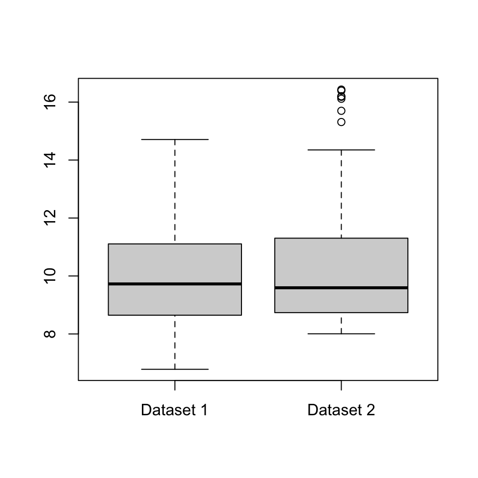
Solution. Some answers could be:
- The median and inter-quartile range of Dataset 2 appear to be very slightly larger than those in Dataset 1, although the differences are very small and might not be important in real life.
- Dataset 2 has a few outliers; Dataset 1 has none.
- While Dataset 1 is fairly “balanced” either side of the median, Dataset 2 shows what statisticians call a “positive skew”: the data above the median is much more spread out than the data below the median.
Group feedback: You can probably think of other answers.
B: Long questions
The next four questions are long questions, which are intended to be harder. Long questions often require you to think originally for yourself, not just directly follow procedures from the notes. You may not be able to solve all of these questions, although you should make multiple attempts to do so. Here, your answers should be written in complete sentences, and you should carefully explain in words each step of your working. Your answers to these questions – not only their mathematical content, but also how to write good, clear solutions – are likely to be the main topic for discussion in your tutorial. Solutions will be available after Friday 13 October.
B1. For each of the two datasets below, calculate the following summary statistics, or explain why it is not possible to do so: mode; median; mean; number of distinct outcomes; inter-quartile range; and sample variance.
(a) Shirt sizes for the \(n = 16\) members of a university football squad:
| Colour | Xtra Small | Small | Medium | Large | Xtra Large |
|---|---|---|---|---|---|
| Number of shirts | 0 | 1 | 6 | 4 | 5 |
Solution. The modal shirt size is medium. The number of distinct outcomes is 4 (we don’t quite “Xtra Small”, which was not observed in the data).
This time, we can order the data from smallest to largest, even though the data is not numerical. Since \((16 + 1)/2 - 8.5\), the median datapoint is the 8th or 9th datapoints, which are Large.
Since \(1 + 0.25(16 - 1) = 4.75\) the lower quartile is the 4th or 5th datapoints, which are Medium. Since \(1 + 0.75(16-1) = 12.25\), the upper quartile is the 12th or 13th datapoints, which are Xtra Large. So we can certainly say that the inner quartiles range from Medium to Xtra Large. We could probably also say that the interquartile range is 3 shirt sizes (Medium, Large, Xtra Large).
Again, because the data is not numerical, we can’t add it up, so can’t calculate a mean or sample variance.
(b) Six packets of Skittles are opened together, a total of \(n = 361\) sweets. The colours of these sweets is recorded as follows:
| Colour | Red | Orange | Yellow | Green | Purple |
|---|---|---|---|---|---|
| Number of Skittles | 67 | 71 | 87 | 74 | 62 |
Solution. The modal colour is Yellow. The number of distinct outcomes is 5.
It’s not possible to calculate the median or the quartiles, because, unlike numerical data, the colours can’t be put “in order” from smallest to largest.
It’s not possible to calculate the mean or sample variance, as these require us to have numerical data that can be “added up”, but this can’t be done with colours.
Group feedback: Make sure your explanation is clear for why we can’t calculate a median for the Skittles data but can for the shirts: the key is whether or not the data can be ordered.
B2. A summary statistic is informally said to be “robust” if it typically doesn’t change much if a small number of outliers are introduced to a large dataset, or “sensitive” if it often changes a lot when a small number of outliers are introduced. Briefly discuss the robustness or sensitivity of the following summary statistics: (a) mode; (b) median; (c) mean; (d) number of distinct outcomes; (e) inter-quartile range; and (f) sample variance.
Solutions.
(a) An outlier will typically be the only data point with its value, or certainly rare. Therefore, the mode will typically not change at all if a small number of outliers are introduced, so is robust. (The exception is for data where every observation is likely to be different, so any outliers become “joint modes” along with everything else; but in this case the mode is not a useful statistic in the first place.)
(b) The introduction of outliers will typically only change the median a little bit, by shifting it between different nearby values in the “central mass” of the data. In particular, the size of the outliers won’t make any difference at all (only whether they are “high outliers” above the median or “low outliers” below the median). So the median is robust.
(c) The mean can change a lot if outliers are introduced, especially if the outlier is enormously far our from the data. So the mean is sensitive.
(d) The number of distinct outcomes will only increase by (at most) 1 for each outlier introduced. This is not typically a relevant increase, so the number of distinct outcomes is robust.
(e) The interquartile range is robust, for the same reason as the median.
(f) The sample variance is sensitive, for the same reason as the mean.
(You might like to think about situations where it’s better to use a robust statistic or better to use a sensitive statistic.)
Group feedback: I find it helpful to suppose I was studying the net worth of people in my tutorial group, and calculating summary statistics. How would those statistics changed change if Elon Musk (owner of Tesla and Twitter, net worth roughly $200 billion) joined my tutorial group? The mean and sample variance would change an enormous amount, while the median and interquartile range would barely change at all in comparison.
Remember that “robust” and “sensitive” are general descriptions rather than precise mathematical definitions. So it doesn’t matter if you disagree with my opinions provided that you give clear and detailed explanations to back up your opinion.
B3. Let \(\mathbf a = (a_1, a_2, \dots a_n)\) and \(\mathbf b = (b_1, b_2, \dots, b_n)\) be two real-valued vectors of the same length. Then the Cauchy–Schwarz inequality says that \[ \left( \sum_{i=1}^n a_i b_i \right)^2 \leq \left( \sum_{i=1}^n a_i^2 \right) \left(\sum_{i=1}^n b_i^2 \right) . \]
(a) By making a clever choice of \((a_i)\) and \((b_i)\) in the Cauchy–Schwarz inequality, show that \(s_{xy}^2 \leq s_x^2 s_y^2\).
Solutions. Recalling the formulas for \(s_{xy}\), \(s_x^2\), and \(s_y^2\), \[\begin{align*} s_{xy} &= \frac{1}{n-1} \sum_{i=1}^n (x_i - \bar x)(y_i - \bar y) ,\\ s_{x}^2 &= \frac{1}{n-1} \sum_{i=1}^n (x_i - \bar x)^2 ,\\ s_{y}^2 &= \frac{1}{n-1} \sum_{i=1}^n (y_i - \bar y)^2 , \end{align*}\] and comparing them with the Cauchy–Schwarz inequality, it looks like taking \(a_i = x_i - \bar x\) and \(b_i = y_i - \bar y\) might be useful.
Making that substitution, we get \[ \left( \sum_{i=1}^n (x_i - \bar x)(y_i - \bar y) \right)^2 \leq \left( \sum_{i=1}^n (x_i - \bar x)^2 \right) \left(\sum_{i=1}^n (y_i - \bar y)^2 \right) . \]
These are very close to the formulas for \(s_{xy}\), \(s_x^2\), and \(s_y^2\), but are just missing the “\(1/(n-1)\)”s; what we in fact have is \[ \left( (n-1) s_{xy} \right)^2 \leq (n-1)s_x^2 \cdot (n-1) s_y^2 .\] Cancelling \((n-1)^2\) from each side, we have \(s_{xy}^2 \leq s_x^2 s_y^2\), as required.
Group feedback: Keep trying different choices for \((a_i)\) and \((b_i)\); maybe your first attempt won’t work, but it pays to be persistent!
A fancier choice is \(a_i = (x_i - \bar x)/\sqrt{n-1}\) and \(b_i = (y_i - \bar y)/\sqrt{n-1}\), to get the exact result without needing a second cancellation step, but I would find that harder to spot.
(b) Hence, show that the correlation \(r_{xy}\) satisfies \(-1 \leq r_{xy} \leq 1\).
Solutions. Recall the formula for the correlation is \[ r_{xy} = \frac{s_{xy}}{s_xs_y} . \] We can make part (a) look a bit like this dividing both sides by \(s_x^2 s_y^2\), to get \[\frac{s_{xy}^2}{s_x^2 s_y^2} \leq 1. \] In fact that’s the square of the correlation on the left-hand side, so we’ve shown that \(r_{xy}^2 \leq 1\).
Finally, we note that if a number squared is less than or equal to 1, then the number must be between -1 and +1 inclusive. (Numbers bigger than 1 get bigger still when squared; numbers smaller than -1 become bigger than +1 when squared; numbers between -1 and +1 get closer to 0.) Hence we have shown that \(-1 \leq r_{xy} \leq 1\), as required.
Group feedback: In part (b) there’s a temptation to “square-root both sides of the inequality”. But you have to be extremely careful if you do this – make sure you are properly accounting for the positive and negative square roots on both sides (if necessary), and where that does or doesn’t require reversing the direction of the inequality. I recommend leaving the square-root operation until the last possible moment of the proof or, perhaps even better, reasoning through words as I did above.
Remember that you can still attempt part (b) even if you got stuck on part (a).
B4. A researcher wishes to study the effect of mental health on academic achievement. The researcher will collect data on the mental health of a cohort of students by asking them to fill in a questionnaire, and will measure academic achievement via the students’ scores on their university exams. Discuss some of the ethical issues associated with the collection, storage, and analysis of this data, and with the publication of the results of the analysis. Are there ways to mitigate these issues?
(It’s not necessary to write an essay for this question – a few short bulletpoints will suffice. There may be an opportunity to discuss these issues in more detail in your tutorial.)
Group feedback: There are no “correct” or “incorrect” answers here, but here are a few things that students in my own tutorials brought up, which may act as a prompt for your own discussions.
It’s important the students/subjects have given their consent for their data to be used this way. It must be “informed consent”, where they understand for what purpose the data will be used, how it will be stored, and so on. It must be easy and painless for students to decline to take part.
Consideration should be given on how to anonymise the data as much as possible – it’s not necessary for those analysing the data to know which questionnaire or which exam result belongs to which student, only that the questionnaire and results can be paired up.
Even if after data is anonymised, care should be taken about whether the students could be worked out from the data. For example, if only one student did a certain combination of modules, their identity could “leak” that way. Perhaps imprecise data, such as classes rather than exact marks, might help maintain privacy while only slightly reducing the usefulness of the data?
On one hand, it seems like this data should perhaps be deleted once analysis has been carried out, for the privacy of the students. On the other hand, principles of “open science” suggest that the data should be kept – and even publicly made available – for other researchers to check the work. There are competing ethical considerations here.
If correlations are found in the data, care should be taken when publishing the analysis not to wrongly suggest a causation. (Just because X and Y are positively correlated, it doesn’t mean that X causes Y – or that Y causes X.)
You can probably think of many other things.
C: Assessed questions
The last two questions are assessed questions. This means you will submit your answers, and your answers will be marked by your tutor. These two questions count for 3% of your final mark for this module. If you get stuck, your tutor may be willing to give you a small hint in your tutorial.
The deadline for submitting your solutions is 2pm on Monday 16 October at the beginning of Week 3. Submission will be via Gradescope, which you can access via Minerva or on the Gradescope mobile app. You should submit your answers as a single PDF file. Most students choose to hand-write their work on paper, then scan-and-submit it to using the Gradescope mobile app. Your work will be marked by your tutor and returned on Monday 23 October, when solutions will also be made available.
Question C1 is a “short question”, where brief explanations or working are sufficient; Question C2 is a “long question”, where the marks are not only for mathematical accuracy but also for the clarity and completeness of your explanatory writing.
You should not collaborate with others on the assessed questions: your answers must represent solely your own work. The University’s rules on academic integrity – and the related punishments for violating them – apply to your work on the assessed questions.
C1. The monthly average exchange rate for US dollars into British pounds over a 12-month period was: \[\begin{gather*} 1.306, \ 1.301, \ 1.290, \ 1.266, \ 1.268, \ 1.302,\\ 1.317, \ 1.304, \ 1.284, \ 1.268, \ 1.247, \ 1.215. \end{gather*}\]
(a) Calculate the median for this data.
(b) Calculate the mean for this data.
(c) Calculate the sample variance for this data.
Hints. Have you checked the definitions of these statistics from Subsection 1.3 of the notes?
(d) Is the mode an appropriate summary statistic for this sort of data? Why/why not?
Hint. Is there a unique mode for this data? Why/why not? For what sort of data does the “mode” give us useful answers?
C2. (a) Suppose that a dataset \(\mathbf x = (x_1, x_2, \dots, x_n)\) (with \(n \geq 2\)) has sample variance \(s_x^2 = 0\). Show that all the datapoints are in fact equal.
Hint. I recommend starting with the definitional formula.
When is the square of something equal to 0? What can you say about the value of a square when it’s nonzero? What can you say about a “sum of squares” – that is, some numbers squared then added together?
(b) Prove the following computational formula for the sample covariance: \[ s_{xy} = \frac{1}{n-1} \left( \sum_{i=1}^n x_iy_i - n\bar x \bar y \right). \]
Hint. In Subsection 1.4 of the notes, we went from the definitional formula for the sample variance to a computational formula. Can you follow a similar argument here?