Problem sheet 3

You should attempt all these questions and write up your solutions in advance of your workshop in week 4 (Monday 15 or Tuesday 16 February) where the answers will be discussed.

1. Consider a Markov chain with state space \(\mathcal S = \{1,2,3\}\), and transition matrix partially given by \[ \mathsf P = \begin{pmatrix} ? & 0.3 & 0.3 \\ 0.2 & 0.4 & ? \\ ? & ? & 1 \end{pmatrix} . \]

(a) Replace the four question marks by the appropriate transition probabilities.

Solution. Rows must add up to 1 and every entry must be non-negative, so the transition matrix is \[ \mathsf P = \begin{pmatrix} 0.4 & 0.3 & 0.3 \\ 0.2 & 0.4 & 0.4 \\ 0 & 0 & 1 \end{pmatrix} . \]

(b) Draw a transition diagram for this Markov chain.

Solution.

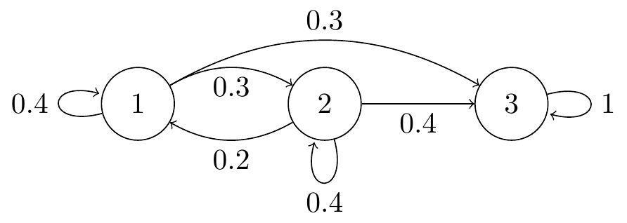
Figure 6.3: Transition diagram for Question 1.

(c) Find the matrix \(\mathsf P(2)\) of two-step transition probabilities.

Solution. \({\displaystyle \mathsf P(2) = \mathsf P^2 = \begin{pmatrix} 0.22 & 0.24 & 0.54 \\ 0.16 & 0.22 & 0.62 \\ 0 & 0 & 1 \end{pmatrix}}\)

(d) By summing the probabilities of all relevant paths, find the three-step transition probability \(p_{13}(3)\).

Solution. There are seven relevant paths: \(1 \to 1 \to 1 \to 3\), \(1 \to 1 \to 2 \to 3\), \(1 \to 1 \to 3 \to 3\), \(1 \to 2 \to 1 \to 3\), \(1 \to 2 \to 2 \to 3\), \(1 \to 2 \to 3 \to 3\), and \(1 \to 3 \to 3 \to 3\). So \[\begin{align*} p_{13}(3) &= p_{11}p_{11}p_{11}p_{13} + p_{11}p_{12}p_{23} + p_{11}p_{13}p_{33} + p_{12} p_{21} p_{13}\\ & \qquad{}+ p_{12}p_{22}p_{23} + p_{12}p_{23}p_{33} + p_{13}p_{33}p_{33}\\ & = 0.4 \cdot 0.4 \cdot 0.3 + 0.4\cdot 0.3\cdot 0.4 + 0.4\cdot 0.3 \cdot 1 + 0.3 \cdot 0.2 \cdot 0.3 \\ & \qquad{}+ 0.3\cdot 0.4 \cdot 0.4 + 0.3 \cdot 0.4 \cdot 1 + 0.3 \cdot 1 \cdot 1\\ &= 0.702 \end{align*}\]

2. Consider a Markov chain \((X_n)\) which moves between the vertices of a tetrahedron.

At each time step, the process randomly chooses one of the edges connected to the current vertex and follows it to a new vertex. The edge to follow is selected randomly with all options having equal probability and each selection is independent of the past movements. Let \(X_n\) be the vertex the process is in after step \(n\).

(a) Write down the transition matrix \(\mathsf P\) of this Markov chain.

The chain can move from a state to any of the other \(3\) states, each with probability \(1/3\). So \[ \mathsf P = \begin{pmatrix} 0 & \frac13 & \frac13 & \frac13 \\ \frac13 & 0 & \frac13 & \frac13 \\ \frac13 & \frac13 & 0 & \frac13 \\ \frac13 & \frac13 & \frac13 & 0 \end{pmatrix} . \]

(b) By summing over all relevant paths of length two, calculate the two-step transition probabilities \(p_{11}(2)\) and \(p_{12}(2)\). Hence, write down the two-step transition matrix \(\mathsf P(2)\).

The length-2 paths from 1 to 1 are \(1 \to k \to 1\) for \(k = 2,3,4\), so \[ p_{11}(2) = p_{12}p_{21} + p_{13}p_{31} + p_{14}p_{41} = \tfrac13 \tfrac13 + \tfrac13 \tfrac13 + \tfrac13 \tfrac13 = \tfrac13 . \] The length-2 paths from 1 to 2 are \(1 \to 3 \to 2\) and \(1 \to 4 \to 2\), so \[ p_{12}(2) = p_{13}p_{32} + p_{14}p_{42} = \tfrac13 \tfrac13 + \tfrac13 \tfrac13 = \tfrac29 . \]

By symmetry, \(p_{ii}(2) = p_{11}(2)\) for all \(i\), and \(p_{ij}(2) = p_{12}(2)\) for all \(i \neq j\). Therefore \[ \mathsf P(2) = \begin{pmatrix} \frac13 & \frac29 & \frac29 & \frac29 \\ \frac29 & \frac13 & \frac29 & \frac29 \\ \frac29 & \frac29 & \frac13 & \frac29 \\ \frac29 & \frac29 & \frac29 & \frac13 \end{pmatrix} . \]

(c) Check your answer by calculating the matrix square \(\mathsf P^2\).

We can verify that \[ \mathsf P^2 = \begin{pmatrix} 0 & \frac13 & \frac13 & \frac13 \\ \frac13 & 0 & \frac13 & \frac13 \\ \frac13 & \frac13 & 0 & \frac13 \\ \frac13 & \frac13 & \frac13 & 0 \end{pmatrix} \begin{pmatrix} 0 & \frac13 & \frac13 & \frac13 \\ \frac13 & 0 & \frac13 & \frac13 \\ \frac13 & \frac13 & 0 & \frac13 \\ \frac13 & \frac13 & \frac13 & 0 \end{pmatrix}= \begin{pmatrix} \frac13 & \frac29 & \frac29 & \frac29 \\ \frac29 & \frac13 & \frac29 & \frac29 \\ \frac29 & \frac29 & \frac13 & \frac29 \\ \frac29 & \frac29 & \frac29 & \frac13 \end{pmatrix} , \] as above.

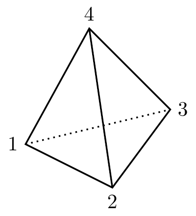
Figure 6.4: A tetrahedron

3. Consider the two-state “broken printer” Markov chain, with state space \(\mathcal S = \{0,1\}\), transition matrix \[ \mathsf P = \begin{pmatrix} 1-\alpha & \alpha \\ \beta & 1-\beta \end{pmatrix} \] with \(0 < \alpha, \beta < 1\), and initial distribution \(\boldsymbol\lambda = (\lambda_0, \lambda_1)\). Write \(\mu_n =\mathbb P(X_n = 0)\).

(a) By writing \(\mu_{n+1}\) in terms of \(\mu_n\), show that we have \[ \mu_{n+1} - \big(1-(\alpha+\beta)\big)\mu_n = \beta . \]

Using the law of total probability, we have \[\begin{multline*} \mathbb P(X_{n+1} = 0) = \mathbb P(X_n = 0)\,\mathbb P(X_{n+1} = 0 \mid X_n = 0) \\ + \mathbb P(X_n = 1)\,\mathbb P(X_{n+1} = 0 \mid X_n = 1) , \end{multline*}\] which in terms of \((\mu_n)\) is \[ \mu_{n+1} = \mu_n (1-\alpha) + (1 - \mu_n)\beta . \] We used here that \(\mathbb P(X_n = 1) = 1-\mu_n\). Rearranging this gives the answer.

(b) By solving this linear difference equation using the initial condition \(\mu_0 = \lambda_0\), or otherwise, show that \[ \mu_n = \frac{\beta}{\alpha+\beta} + \left(\lambda_0 - \frac{\beta}{\alpha+\beta}\right)\big(1-(\alpha+\beta)\big)^n . \]

The characteristic equation is \(\lambda - (1-(\alpha+\beta)) = 0\) with a single root at \(\lambda = 1 - (\alpha+\beta)\). The general solution to the homogeneous equation is, therefore, \(A(1-(\alpha+\beta))^n\).

For a particular solution, we guess a solution \(\mu_n = C\), and \(C - (1-(\alpha+\beta))C = \beta\) gives \(C = \beta/(\alpha+\beta)\). Thus the general solution to the inhomogeneous equation is \[ \mu_n = \frac{\beta}{\alpha+\beta} + A\big(1-(\alpha+\beta)\big)^n .\]

From the initial condition, we get \(\lambda_0 = \beta/(\alpha+\beta) + A\), and therefore \(A = \lambda_0 - \beta/(\alpha+\beta)\). The solution is therefore as given.

(c) What, therefore, are \(\lim_{n\to\infty} \mathbb P(X_n = 0)\) and \(\lim_{n\to\infty} \mathbb P(X_n = 1)\)?

Note that \(-1 < 1 - (\alpha + \beta) < 1\), so \((1-(\alpha+\beta))^n \to 0\). Therefore we have \[\begin{align*} \lim_{n\to\infty} \mathbb P(X_n = 0) &= \lim_{n\to\infty} \mu_n \\ &= \lim_{n\to\infty} \left( \frac{\beta}{\alpha+\beta} + \left(\lambda_0 - \frac{\beta}{\alpha+\beta}\right)\big(1-(\alpha+\beta)\big)^n \right) \\ &= \frac{\beta}{\alpha+\beta} . \end{align*}\] Since \(\mathbb P(X_n = 1) = 1- \mathbb P(X_n = 0)\), we have \[ \mathbb P(X_n = 1) \to 1 - \frac{\beta}{\alpha+\beta} = \frac{\alpha}{\alpha+\beta} . \]

(d) Explain what happens if the Markov chain is started in the distribution \[ \lambda_0 = \frac{\beta}{\alpha+\beta} , \qquad \lambda_1 = \frac{\alpha}{\alpha+\beta} . \]

Substituting in the value of \(\lambda_0\) into the equation for \(\mu_n\), the second term cancel, and we have that \(\mathbb P(X_n = 0) = \mu_n = \beta/(\alpha+\beta)\) for all times \(n\), and therefor \(\mathbb P(X_n = 1) = \alpha/(\alpha+\beta)\) too. This means that the Markov chain remains in the same “stationary distribution” forever.

4. Let \((X_n)\) be a Markov chain. Show that, for any \(m \geq 1\), we have \[ \mathbb P(X_{n+m} = x_{n+m} \mid X_n = x_n, X_{n-1} = x_{n-1}, \dots, X_0 = x_0) = \mathbb P(X_{n+m} = x_{n+m} \mid X_n = x_n) . \]

Note that we have a sequence of statements here, for \(m = 1, 2, \dots\). Note also that the case \(m = 1\) is the standard Markov property. When we have a sequence of statements and we can easily prove the first one, this is a good sign that a proof by induction is the way to go.

Before starting, for reasons of space, we adopt notation where we suppress the capital \(X\)s, so we want to show that \[ \mathbb P(x_{n+m} \mid x_n, x_{n-1}, \dots, x_0 ) = \mathbb P(x_{n+m} \mid x_n) . \]

We work by induction on \(m\). The base case \(m = 1\) is the standard Markov property.

Assume the inductive hypothesis: that result holds for \(m\). We now need to prove the inductive step: that the result holds for \(m+1\). For \(m+1\) we have, by conditioning on the first step \(x_{n+1}\), \[\begin{multline*} \mathbb P(x_{n+m+1} \mid x_n, x_{n-1}, \dots, x_0 ) \\ = \sum_{x_{n+1}} \mathbb P(x_{n+1} \mid x_n, x_{n-1}, \dots, x_0 )\,\mathbb P(x_{n+m+1} \mid x_{n+1}, x_n, x_{n-1}, \dots, x_0 ) \end{multline*}\] By the standard Markov property the first term simplifies to \(\mathbb P(x_{n+1} \mid x_n)\), and by the result for \(m\) the second term simplifies to \(\mathbb P(x_{n+m+1} \mid x_{n+1})\). So we have \[ \mathbb P(x_{n+m+1} \mid x_n, x_{n-1}, \dots, x_0 ) = \sum_{x_{n+1}} \mathbb P(x_{n+1} \mid x_n) \mathbb P(x_{n+m+1} \mid x_{n+1}) . \] But the right-hand side here is \(\mathbb P(x_{n+m+1} \mid x_n)\) written using conditioning on the first step and using the result for \(m\). By induction, we are done.

5. A car insurance company operates a no-claims discount system for existing policy holders. The possible discounts on premiums are \(\{0\%,25\%,40\%,50\%\}\). Following a claim-free year, a policyholder’s discount level increases by one level (or remains at 50% discount). If the policyholder makes one or more claims in a year, the discount level decreases by one level (or remains at 0% discount).

The insurer believes that the probability of of making at least one claim in a year is \(0.1\) if the previous year was claim-free and \(0.25\) if the previous year was not claim-free.

(a) Explain why we cannot use \(\{0\%,25\%,40\%,50\%\}\) as the state space of a Markov chain to model discount levels for policyholders.

The Markov property does not hold for the time-homogeneous process described since the probability of moving to a given state at the next time step is not simply dependent on the current state if \(\mathcal S=\{0\%,25\%,40\%,50\%\}\). For example, \[ \mathbb P(X_{n+1}=25\% \mid X_n= 40\% )=\begin{cases} 0.25 & \text{if $X_{n-1}=50\%$}\\ 0.1 & \text{if $X_{n-1}=25\%$.} \end{cases} \]

(b) By considering additional states, show that a Markov chain can be used to model the discount level.

The problem is that the process has a memory of the previous year. If we currently have a discount of 0%, we know a claim was made in the year before, so no changes are required. Similarly, at 50% discount, we know that no claim was made in the previous year. The other two states, 25% and 40%, have different behaviour depending on whether or not there was a claim in the previous year.

So we will split each of these into two states: 25+ will denote a 25% discount with no claim in the previous year, while 25- will denote a 25% discount with a claim in the previous year. We define the state 40+ and 40- similarly. Then we have a Markov chain, since the current state and the number of claims in the previous year completely defines the distribution on future behaviour.

(c) Draw the transition diagram and write down the transition matrix.

The transition diagram is as shown below.

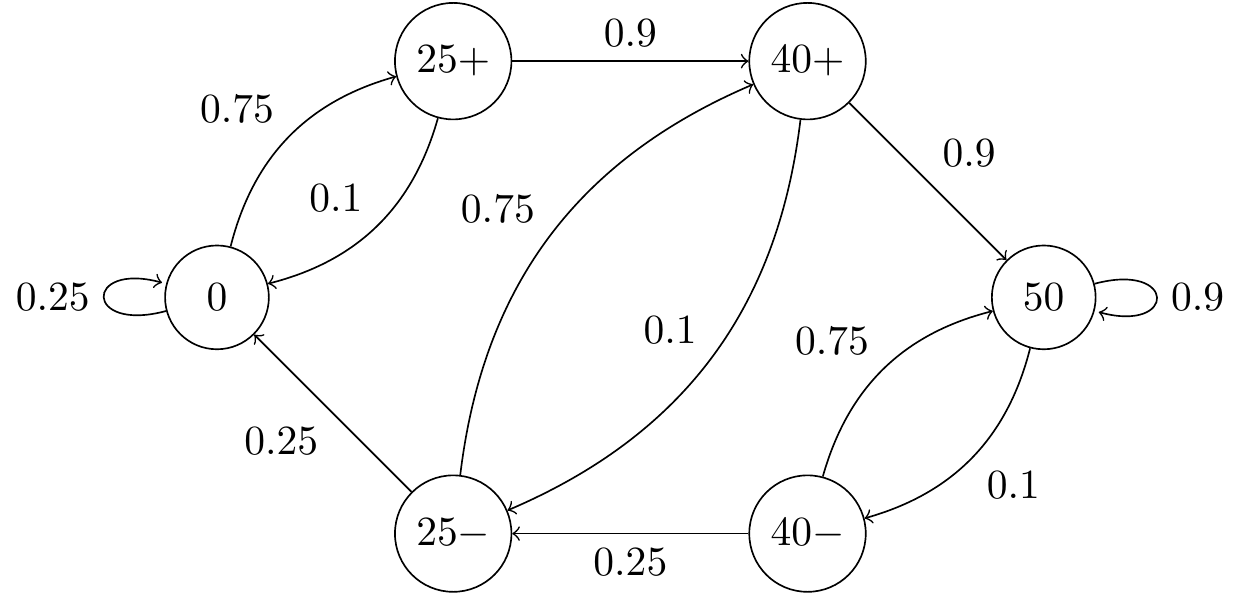
Figure 6.5: Transition diagram for the car insurance Markov chain

The transition matrix is given by, \[ \mathsf P = \begin{matrix} & \begin{matrix} 0 & 25+ & 25- & 40+ & 40- & 50 \end{matrix} \\ \begin{matrix} 0 \\ 25+ \\ 25- \\ 40+ \\ 40- \\ 50 \end{matrix} & \begin{pmatrix} 0.25 & 0.75 & 0 & 0 & 0 & 0 \\ 0.1 & 0 & 0 & 0.9 & 0 & 0 \\ 0.25 & 0 & 0 & 0.75 & 0 & 0 \\ 0 & 0 & 0.1 & 0 & 0 & 0.9 \\ 0 & 0 & 0.25 & 0 & 0 & 0.75 \\ 0 & 0 & 0 & 0 & 0.1 & 0.9 \end{pmatrix} \end{matrix} \]

6. The credit rating of a company can be modelled as a Markov chain. Assume the rating is assessed once per year at the end of the year and possible ratings are A (good), B (fair) and D (in default). The transition matrix is \[\mathsf P=\begin{pmatrix} 0.92&0.05&0.03\\ 0.05&0.85&0.1\\ 0&0&1 \end{pmatrix} . \]

(a) Calculate the two-step transition probabilities, and hence find the expected number of defaults in the next two years from \(100\) companies all rated A at the start of the period.

The matrix of two-step transition probabilities is given by the matrix square \[\mathsf P(2) = \mathsf P^2= \begin{pmatrix} 0.8489&0.0885&0.0626\\ 0.0885&0.7250&0.1865\\ 0&0&1 \end{pmatrix}. \] The number of defaults in two years from \(100\) A-rated companies is \(100 \times p_{\mathrm{AD}}(2) = 100 \times 0.0626 = 6.26\).

(b) What is the probability that a company rated A will at some point default without ever having been rated B in the meantime?

Let \(\delta\) be the desired probability that an A-rated company will default without having been rated B. We condition on the first step: with probability \(0.92\) we remain in state A, and by the Markov property the probability of the given event remains at \(\delta\); with probability \(0.05\) we move to state B, and the event fails to occur; and with probability \(0.03\) we move to state D and the event occurs immediately. Therefore, we have \[ \delta = 0.92\delta + 0.05\times 0 + 0.03 \times 1 = 0.92\delta + 0.03 , \] which has solution \(\delta = 0.03/(1-0.92) = 0.375\).

A corporate bond portfolio manager follows an investment strategy which means that bonds which fall from A-rated to B-rated are sold and replaced with an A-rated bond. The manager believes this will improve the returns on the portfolio because it will reduce the number of defaults experienced.

(c) Calculate the expected number of defaults in the manager’s portfolio over the next two years given there are initially 100 A-rated bonds.

Given that B-rated bonds are replaced by A-rated bonds, we have a new Markov chain with state space \(\{\mathrm{A},\mathrm{D}\}\) and transition matrix \[ \mathsf P = \begin{pmatrix} 0.92+0.05 & 0.03 \\ 0 & 1 \end{pmatrix} = \begin{pmatrix} 0.97 & 0.03 \\ 0 & 1 \end{pmatrix} . \] The two-step transition probability is \[ \mathsf P(2) = \mathsf P^2 = \begin{pmatrix} 0.97 & 0.03 \\ 0 & 1 \end{pmatrix} \begin{pmatrix} 0.97 & 0.03 \\ 0 & 1 \end{pmatrix} = \begin{pmatrix} 0.9409 & 0.0591 \\ 0 & 1 \end{pmatrix} . \] Thus the number of defaults from \(100\) A-rated bonds in two years is \(100\times p_{\mathrm{AD}}(2) = 100\times 0.0591 = 5.91\). The manager was right: this is slightly less than the \(6.26\) from part (a).