Section 14 Poisson process with exponential holding times

Reminder: the exponential distribution
The Poisson process has exponential holding times
The Markov property in continuous time

14.1 Exponential distribution

Last time, we introduced the Poisson process by looking at the random number of arrivals in fixed amount of time, which follows a Poisson distribution. Another way of looking at the Poisson process is to look at the random amount of of time required for a fixed number of arrivals. For this, we’ll need the exponential distribution.

We start by recalling the exponential distribution. Recall that we say a continuous random variable $T$ has the exponential distribution with rate $\lambda$, and write $T \sim \operatorname{Exp}(\lambda)$, if it has the probability distribution function $f(t) = \lambda \mathrm{e}^{-\lambda t}$ for $t \geq 0$.

Exponential distributions are often used to model “waiting times” – for example, the amount of time until a light bulb breaks, the times between buses arriving, or the time between withdrawals from a bank account.

You are reminded of the following facts about the exponential distribution:

The cumulative distribution function is $F(t) = \mathbb P(T \leq t) = 1 - \mathrm{e}^{-\lambda t}$; although it is usually more convenient to deal with the tail probability $\mathbb P(T > t) = 1 - F(t) = \mathrm{e}^{-\lambda t}$.
The expectation is $\mathbb E T = 1/\lambda$ and the variance is $\operatorname{Var}(T) = 1/\lambda^2$.

The following memoryless property will of course be important in a course about memoryless Markov processes.

Theorem 14.1 Let $T \sim \operatorname{Exp}(\lambda)$. Then, for any $s,t\geq0$, \[ \mathbb P(T > t + s \mid T > t) = \mathbb P(T > s) . \]

Suppose we are waiting an exponentially distributed time for an alarm to go off. No matter how long we’ve been waiting for, the remaining time to wait is still exponentially distributed, with the same parameter – hence “memoryless”.

Proof. By standard use of conditional probability, we have \[ \mathbb P(T > t + s \mid T > t) = \frac{\mathbb P(T > t + s \text{ and } T > t)}{\mathbb P(T > t)} = \frac{\mathbb P(T > t + s)}{\mathbb P(T > t)} = \frac{\mathrm{e}^{-\lambda(t+s)}}{\mathrm{e}^{-\lambda t}} = \mathrm{e}^{-\lambda s} , \] which is still the tail probability of the exponential distribution.

The following property will be important later on in the course.

Theorem 14.2 Let $T_1 \sim \operatorname{Exp}(\lambda_1)$, $T_2 \sim \operatorname{Exp}(\lambda_2)$, $\dots$, $T_n \sim \operatorname{Exp}(\lambda_n)$ be independent exponential distributions, and let $T$ be the minimum of the $T_i$s, so $T = \min\{T_1, T_2, \dots, T_n \}$. Then \[ T \sim \operatorname{Exp}(\lambda_1 + \lambda_2 + \cdots + \lambda_n) . \] Further, the probability that $T_j$ is the smallest of all the $T_i$s is \[ \mathbb P(T = T_j) = \frac{\lambda_j}{\lambda_1 + \lambda_2 + \cdots + \lambda_n} . \]

Proof. The proof of this is an question on Problem Sheet 7.

14.2 Definition 2: exponential holding times

We mentioned before that exponential distributions are often used to model “waiting times”. When modelling a process $(X(t))$ counting many arrivals at rate $\lambda$, we might model the process like this: after waiting an $\operatorname{Exp}(\lambda)$ amount of time, an arrival appears. After another $\operatorname{Exp}(\lambda)$ amount of time, another arrival appears. And so on. We often use the term “holding time” to refer to the time between consecutive arrivals.

This suggests a process with the following properties:

We start with $X(0) = 0$.
Let $T_1, T_2, \dots \sim \operatorname{Exp}(\lambda)$ be the holding times, all independent. Then \[ X(t) = \begin{cases} 0 & \text{for $0 \leq t < T_1$} \\ 1 & \text{for $T_1 \leq t < T_1 + T_2$} \\ 2 & \text{for $T_1+T_2 \leq t < T_1 + T_2 + T_3$} \\ \text{and so on.} & \end{cases} \]

A process described like this is also the Poisson process!

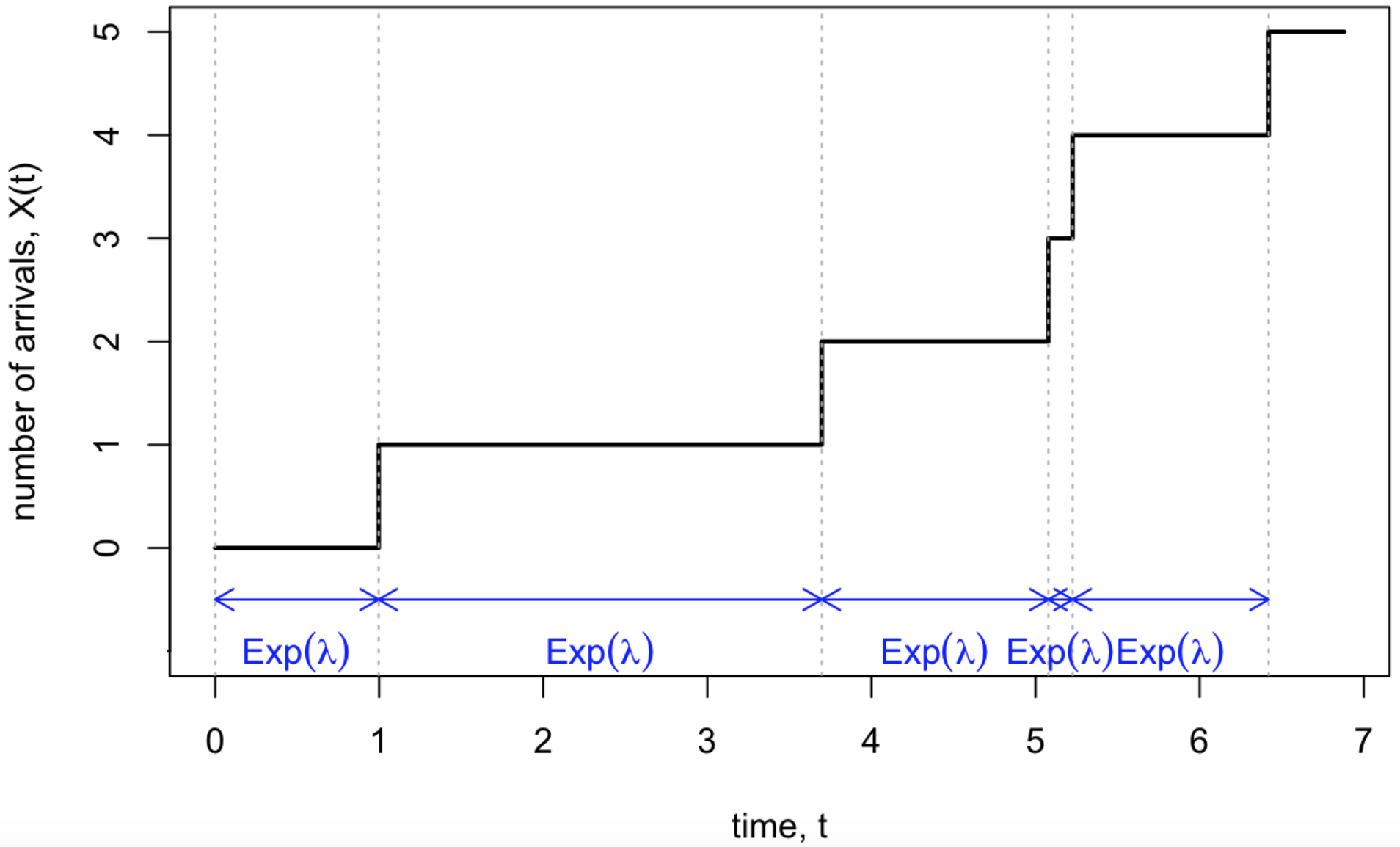
Figure 14.1: A Poisson process with exponentially distributed holding times.

Theorem 14.3 Let $(X(t))$ be a Poisson process with rate $\lambda$, as defined by its independent Poisson increments (see Subsection 13.2). Then $(X(t))$ has the exponential holding times structure described above.

Proof. Let $(X(t))$ be a Poisson process with rate $\lambda$. We seek the distribution of the first arrival time $T_1$. We have \[ \mathbb P(T_1 > t_1) = \mathbb P\big(X(t_1) - X(0) = 0\big) = \mathrm{e}^{-\lambda t_1} \frac{(\lambda t_1)^0}{0!} = \mathrm{e}^{-\lambda t_1} , \] since the arrival comes after $t_1$ if there are no arrivals in the interval $[0,t_1]$. But this is precisely the tail probability of an exponential distribution with rate $\lambda$.

Now consider the second holding time. We have \[ \mathbb P(T_2 > t_2 \mid T_1 = t_1) = \mathbb P\big(X(t_1 + t_2) - X(t_1) = 0\big) = \mathrm{e}^{-\lambda ((t_1 + t_2) - t_1)} = \mathrm{e}^{-\lambda t_2} \] by the same argument as before. This is the tail distribution for another $\operatorname{Exp}(\lambda)$ distribution, independent of $T_1$.

Repeating this argument for all $n$ gives the desired exponential holding time structure.

Example 14.1 Customers visit a second-hand bookshop at a rate of $\lambda = 5$ per hour. Each customer a book with probability $p = 0.4$. What is the expected time to make ten sales, and what is the standard deviation?

The count of books sold marked Poisson process, which we saw last time is itself a Poisson process with rate $p\lambda = 2$.

The expected time of the tenth sale is \[ \mathbb E(T_1 + \dots + T_{10}) = 10\,\mathbb ET_1 = 10 \times \tfrac{1}{2} = 5 \text{ hours} .\] The variance is \[ \operatorname{Var}(T_1 + \dots + T_{10}) = 10\,\operatorname{Var}(T_1) = 10 \times \frac{1}{2^2} = 2.5 , \] where we used that the holding times are independent and identically distributed, so the standard deviation is $\sqrt{2.5} = 1.58$ hours.

What is the probability it takes more than an hour to sell the first book?

This is the probability the first holding time is longer than an hour, which is the tail of the exponentital distribution, \[ \mathbb P(T_1 > 1) = \mathrm{e}^{-2\times 1} = \mathrm{e}^{-2} = 0.135. \]

An alternative way to solve this would be to say that the first book is is sold later than 1 hour in if $X(1) = 0$. So using the Poisson increments definition from last time, we have \[ \mathbb P\big(X(1) = 0\big) = \mathrm{e}^{-2\times 1} \frac{(2\times 1)^0}{0!} = \mathrm{e}^{-2} = 0.135. \] We get the same answer either way.

14.3 Markov property in continuous time

We previously saw the Markov “memoryless” property in discrete time. The equivalent definition in continuous time is the following.

Definition 14.1 Let $(X(t))$ be a stochastic process on a discrete state space $\mathcal S$ and continuous time $t \in [0,\infty)$. We say that $(X(t))$ has the Markov property if \[\begin{multline*} \mathbb P\big( X(t_{n+1}) = x_{n+1} \mid X(t_n) = x_n, \dots, X(t_1) = x_1, X(t_0) = x_0 \big) \\ = \mathbb P\big( X(t_{n+1}) = x_{n+1} \mid X(t_n) = x_{n}\big) \end{multline*}\] for all times $t_0 < t_1 < \cdots < t_n < t_{n+1}$ and all states $x_0, x_1, \dots, x_n, x_{n+1} \in \mathcal S$.

In other words, the state of the process at some point $t_{n+1}$ in the future depends on where we are now $t_n$, but, given that, does not depend on any collection of previous times $t_0, t_1, \dots, t_{n-1}$.

The Poisson process does indeed have the Markov property, since, by the property of independent increments, we have that \[ \mathbb P\big( X(t_{n+1}) = x_{n+1} \mid X(t_n) = x_n, \dots, X(t_0) = x_0 \big) = \mathbb P\big( X(t_{n+1}) -X(t_n) = x\big) , \] where $x = x_{n+1}-x_n$. By Poisson increments, this has probability \[ \mathrm{e}^{-\lambda(t_{n+1}-t_n)} \frac{\big(\lambda(t_{n+1}-t_n)\big)^x}{x!} . \]

Alternatively, by the memoryless property of the exponential distribution, we see that we can restart the holding time from $t_n$ and still have this and all future holding times exponentially distributed.

In the next section, we look at the Poisson process in a third way, by looking at what happens in a very small time period.