Section 11 Long-term behaviour of Markov chains

The limit theorem: convergence to the stationary distribution for irreducible, aperiodic, positive recurrent Markov chains
The ergodic theorem for the long-run proportion of time spent in each state

11.1 Convergence to equilibrium

In this section we’re interested in what happens to a Markov chain $(X_n)$ in the long-run – that is, when $n$ tends to infinity.

One thing that could happen over time is that the distribution $\mathbb P(X_n = i)$ of the Markov chain could gradually settle down towards some “equilibrium” distribution. Further, perhaps that long-term equilibrium might not depend on the initial distribution, but the effects of the initial distribution might eventually almost disappear, exhibiting a “lack of memory” of the start of the process.

Just in case that does happen, let’s give it a name.

Definition 11.1 Let $(X_n)$ be a Markov chain on a state space $\mathcal S$ with transition matrix $\mathsf P$. Suppose there exists a distribution $\mathbf p^* = (p_i^*)$ on $\mathcal S$ (so $p_i^* \geq 0$ and $\sum_i p_i^* = 1$) such that, whatever the initial distribution $\boldsymbol\lambda = (\lambda_i)$, we have $\mathbb P(X_n = j) \to p^*_j$ as $n \to \infty$ for all $j \in \mathcal S$. Then we say that $\mathbf p^*$ is an equilibrium distribution.

It’s clear there can only be at most one equilibrium distribution – but will there be one at all? The following is the most important result in this course. (Recall that an irreducible Markov chain is aperiodic if it has period 1.)

Theorem 11.1 (Limit theorem) Let $(X_n)$ be an irreducible and aperiodic Markov chain. Then for any initial distribution $\boldsymbol\lambda$, we have that $\mathbb P(X_n = j) \to 1/\mu_j$ as $n \to \infty$, where $\mu_j$ is the expected return time to state $j$.

In particular:

Suppose $(X_n)$ is positive recurrent. Then the unique stationary distribution $\boldsymbol\pi$ given by $\pi_j = 1/\mu_j$ is the equilibrium distribution, so $\mathbb P(X_n = j) \to \pi_j$ for all $j$.
Suppose $(X_n)$ is null recurrent or transient. Then $\mathbb P(X_n = j) \to 0$ for all $j$, and there is no equilibrium distribution.

I particularly like how this one theorem gathers together all the ideas from the course in one result (Markov chains, irreducibility, periodicity, recurrence/transience, positive/null recurrence, return times, stationary distribution…).

Note the three conditions for convergence to an equilibrium distribution: irreducibility, aperiodicity, and positive recurrence.

Consider a irreducible, aperiodic, positive recurrent Markov chain. Taking the initial distribution to be starting in state $i$ with certainty, the limit theorem tells us that $p_{ij}(n) \to \pi_j$ for all $i$ and $j$. This means that the $n$-step transition matrix will have the limiting value \[ \lim_{n \to \infty} \mathsf P(n) = \begin{pmatrix} \pi_1 & \pi_2 & \cdots & \pi_N \\ \pi_1 & \pi_2 & \cdots & \pi_N \\ \vdots & \vdots & \vdots & \vdots \\ \pi_1 & \pi_2 & \cdots & \pi_N \end{pmatrix} , \] where each row is identical.

We give an full proof of the limit theorem below (optional and nonexaminable). However, this easier result gets part way there.

Theorem 11.2 If an equilibrium distribution $\mathbf p^*$ does exist, then $\mathbf p^*$ is a stationary distribution.

Given this result it’s clear that an irreducible Markov chain cannot have an equilibrium distribution if it is null recurrent or transient, as it doesn’t even have a stationary distribution. So the positive recurrent case is the hard (nonexaminable) one.

Proof. We need to verify that $\mathbf p^* \mathsf P = \mathbf p^*$. We have \[ \sum_i p_i^* p_{ij} = \sum_i \left(\lim_{n\to\infty} p_{ki}(n) \right) p_{ij} = \lim_{n\to\infty} \sum_i p_{ki}(n) p_{ij} = \lim_{n\to\infty} p_{kj}(n+1) = p^*_j , \] as desired.

(Strictly speaking, swapping the sum and the limit is only formally justified when the state space is finite, although the theorem is true universally.)

11.2 Examples of convergence and non-convergence

Example 11.1 The two-state “broken printer” Markov chain is irreducible, aperiodic, and positive recurrent, so its stationary distribution is also the equilibrium distribution. We proved this from first principles in Question 3 on Problem Sheet 3.

Example 11.2 Recall the simple no-claims discount Markov chain from Lecture 6, which is irreducible, aperiodic, and positive recurrent. We saw last time that is has the unique stationary distribution \[ \boldsymbol\pi = \left(\tfrac1{13} \quad \tfrac{3}{13}\quad \tfrac9{13}\right) = (0.0769\quad 0.2308\quad 0.6923) . \]

From the limit theorem, we see that the $n$-step transition probability tends to a limit where every row is equal to $\boldsymbol\pi$. We can check using a computer: for $n = 12$, say, \[ \mathsf P(12) = \mathsf P^{12} = \begin{pmatrix} 0.0770 & 0.2308 & 0.6923 \\ 0.0769 & 0.2308 & 0.6923 \\ 0.0769 & 0.2308 & 0.6923 \end{pmatrix}, \] where $p_{ij}(12)$ is equal to $\pi_j$ up to at least 3 decimal places for all $i,j$. As $n$ gets bigger, the matrix gets closer and closer to the limiting form.

Example 11.3 The simple random walk is null recurrent for $p = \frac12$ and transient otherwise. Either way, we have $\mathbb P(X_n = i) \to 0$ for all states $i$, and there is no equilibrium distribution.

Example 11.4 Consider a Markov chain $(X_n)$ on state space $\mathcal S = \{0,1\}$ and transition matrix \[ \mathsf P = \begin{pmatrix} 0 & 1 \\ 1 & 0 \end{pmatrix} . \] So at each stage we swap from state $0$ to state $1$ and back again. This chain is irreducible and positive recurrent, so it has a unique stationary distribution, which is clearly $\boldsymbol\pi = (\frac12\quad\frac12)$.

However, we don’t have convergence to equilibrium. If we start from initial distribution $(\lambda_0, \lambda_1)$, then $\mathbb P(X_n = 0) = \lambda_0$ for even $n$ and $\mathbb P(X_n = 0) = \lambda_1$ for odd $n$. When $\lambda_0 \neq \frac12$, this does not converge.

The point is that this chain is not aperiodic: it has period $2$, so the limit theorem does not apply.

Example 11.5 Consider a Markov chain with state space $\mathcal S = \{1,2,3\}$ and transition diagram as shown below.

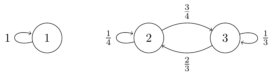
Figure 11.1: Transition diagram for a Markov chain with two positive recurrent classes.

This chain is not irreducible, but has two aperiodic and positive recurrent communicating classes. In particular, it has many stationary distributions including $(1, 0, 0)$ and $(0, \frac8{17}, \frac9{17})$ (optional exercise for the reader). If we start in state 1, then the limiting distribution is the former, while if we start in states 2 or 3, the limiting distribution is the latter.

In particular, as $n \to \infty$, we have \[ \mathsf P^{(n)} \to \begin{pmatrix} 1 & 0 & 0 \\ 0 & \frac8{17} & \frac9{17} \\ 0 & \frac8{17} & \frac9{17} \end{pmatrix}. \]

11.3 Ergodic theorem

The limit theorem looked at the limit of $\mathbb P(X_n = j)$, the probability that the Markov chain is in state $j$ at some specific point in time $n$ a long time in the future. We could also look at the long-run amount of time spent in state $j$; that is, averaging the behaviour over a long time period. (The word “ergodic” is used in mathematics to refer to concepts to do with the long-term proportion of time.)

Let us write \[ V_j(N) := \# \big\{ n < N : X_n = j \} \] for the total number of visits to state $j$ up to time $N$. Then we can interpret $V_j(n)/n$ as the proportion of time up to time $n$ spent in state $j$, and its limiting value (if it exists) to be the long-run proportion of time spent in state $j$.

Theorem 11.3 (Ergodic theorem) Let $(X_n)$ be an irreducible Markov chain. Then for any initial distribution $\boldsymbol\lambda$ we have that $V_j(n)/n \to 1/\mu_j$ almost surely as $n \to \infty$, where $\mu_j$ is the expected return time to state $j$.

In particular:

Suppose $(X_n)$ is positive recurrent. Then there is a unique stationary distribution $\boldsymbol\pi$ given by $\pi_j = 1/\mu_j$, and $V_j(n)/n \to \pi_j$ almost surely for all $j$.
Suppose $(X_n)$ is null recurrent or transient. Then $V_j(n)/n \to 0$ almost surely for all $j$.

For completeness, we should note that “almost sure” convergence means that $\mathbb P(V_j(n)/n \to 1/\mu_j) = 1$, although the precise definition is not important for us in this module.

Note that, because we are averaging over a long-time period, we no longer need the condition that the Markov chain is aperiodic; for convergence of the long-term proportion of time to the stationary distribution we just need irreducibility and positive recurrence.

Again, we give an optional and nonexaminable proof below.

Example 11.6 Recall the simple no-claims discount Markov chain. Since this chain is irreducible and positive recurrent, we now see that the long-term proportion of time spent in each state corresponds to the stationary distribution $\boldsymbol\pi = (\frac1{13} \quad \frac{3}{13}\quad \frac9{13})$. Therefore, over the lifetime of an insurance policy held for a long period of time, the average discount is approximately \[ \tfrac{1}{13}(0\%) + \tfrac{3}{13}(25\%) + \tfrac{9}{13}(50\%) = \tfrac{21}{52} = 40.4\% . \]

Example 11.7 The two-state “swapping” chain we saw earlier did have a unique stationary distribution $(\frac12, \frac12)$, but did not have an equilibrium distribution, because it was periodic. But it is true that $V_0(n)/n \to \pi_0 = \frac12$ and $V_1(n)/n \to \pi_1 = \frac12$, due to the ergodic theorem. So although where we are at some specific point in the future depends on where we started from, in the long run we always spend half our time in each state.

11.4 Proofs of the limit and ergodic theorems

This subsection is optional and nonexaminable.

Again, it’s important to be able to use the limit and ergodic theorems, but less important to be able to prove them.

First, the limit theorem. The only bit left is the first part: that for an irreducible, aperiodic, positive recurrent Markov chain, the stationary distribution $\boldsymbol\pi$ is an equilibrium distribution.

This cunning proof uses a technique called “coupling”. When looking at two different random objects $X$ and $Y$ (like random variables or stochastic processes), it seems natural to prefer $X$ and $Y$ to be independent. However, coupling is the idea that it can sometimes be beneficial to let $X$ and $Y$ actually be dependent on each other.

Proof (Proof of Theorem 11.1). Let $(X_n)$ be our irreducible, aperiodic, positive recurrent Markov chain with transition matrix $\mathsf P$ and initial distribution $\boldsymbol\lambda$. Let $(Y_n)$ be a Markov chain also with transition matrix $\mathsf P$ but “in equilibrium” – that is, started from the stationary distribution $\boldsymbol\pi$, and thus staying in that distribution for ever.

Pick a state $s \in \mathcal S$, and let $T$ be the first time the $X_n = Y_n = s$ (or $T = \infty$, if that never happens). Now here’s the coupling: after $T$, when $(X_n)$ and $(Y_n)$ collide at $s$, then make $(X_n)$ stick to $(Y_n)$, so $X_n = Y_n$ for $n \geq T$. Since a Markov chain has no memory, $(X_{T+n}) = (Y_{T+n})$ is still just a Markov chain with the same transition probabilities from that point on. (Readers of a previous optional subsection will recognise $T$ as a stopping time and will notice we’re using the strong Markov property.) Most importantly, thanks to the coupling, from the time $T$ onwards, $(X_n)$ will also always have distribution $\boldsymbol\pi$, a fact that will obviously be very useful in this proof.

It will be important that $T$ is finite with probability 1. Define $(\mathbf Z_n)$ by $\mathbf Z_n = (X_n, Y_n)$. So $(\mathbf Z_n)$ is a Markov chain on $\mathcal S \times \mathcal S$, and $T$ is the expected hitting time of $(\mathbf Z_n)$ to the state $(s, s) \in \mathcal S \times \mathcal S$. The transition probabilities for $(\mathbf Z_n)$ are $\mathsf{\tilde P} = (\tilde p_{(i,k)(j,l)})$ where \[ \tilde p_{(i,k)(j,l)} = p_{ij}p_{kl} . \] This is the probability that the joint chain goes from $\mathbf Z_n = (X_n, Y_n) = (i, k)$ to $\mathbf Z_{n+1} = (X_{n+1}, Y_{n+1}) = (j, l)$.

Since the original Markov chain is irreducible and aperiodic, this means that $p_{ij}(n), p_{kl}(n) > 0$ for all $n$ sufficiently large, so $\tilde p_{(i,k)(j,l)}(n) > 0$ for all $n$ sufficiently large also, meaning that $(\mathbf Z_n)$ is irreducible (and, although this isn’t required, aperiodic). Further, $(\mathbf Z_n)$ has a stationary distribution $\mathbf{\tilde \pi} = (\tilde \pi_{(i,k)})$ where \[ \tilde \pi_{(i,k)} = \pi_i \pi_k , \] which means that $(\mathbf Z_n)$ is positive recurrent. Thus $T$ is finite with probability 1.

So we can finally prove the limit theorem. We want to show that $\mathbb P(X_n = i)$ tends to $\pi_i$. The difference between them is \[\begin{align*} \big|\mathbb P(X_i = i) - \pi_i\big| &= \mathbb P(n \leq T)\times\big|\mathbb P(X_i = i \mid n \leq T) - \pi_i\big| + P(n > T) \times |\pi_i - \pi_i| \\ &= \mathbb P(n \leq T)\times\big|\mathbb P(X_i = i \mid n \leq T) \\ &\leq \mathbb P(n \leq T) . \end{align*}\] Here, the equality on the first line is because $(X_n)$ follows the stationary distribution exactly once it sticks to $(Y_n)$ after time $T$, and the inequality on the third line is because the absolute difference between two probabilities is between 0 and 1. But we’ve already shown that $T$ is finite with probability 1, so $\mathbb P(n \leq T) = \mathbb P(T \geq n) \to 0$, and we’re done.

The proof of the ergodic theorem uses the law of large numbers. Recall that the law of large numbers states that if $Y_1, Y_2, \dots$ are IID random variables with mean $\mu$, then \[ \frac{Y_1 + Y_2 + \cdots + Y_n}{n} \to \mu \qquad \text{as $n \to \infty$}. \] This means it’s also true that for any sequence $(a_n)$ with $a_n \to \infty$, we also have \[ \frac{Y_1 + Y_2 + \cdots + Y_{a_n}}{a_n} \to \mu \qquad \text{as $n \to \infty$}. \]

Proof (Proof of Theorem 11.3). If $(X_n)$ is transient, then the number of visits to state $i$ is finite with probability 1, so $V_i(n)/n \to 0$, as required.

Suppose instead that $(X_n)$ is recurrent. By our useful lemma we know we will hit $i$ in finite time, so we can ignore that negligible “burn-in” period, and (by the strong Markov property) assume we start from $i$. Let $M_{i}^{(r)}$ be the time between the $r$th and $(r+1)$th visits to $i$. Note that the $M_{i}^{(r)}$ are IID with mean $\mu_i$.

The time of the last visit to $i$ before time $n$ is \[ M_{i}^{(1)} + M_{i}^{(2)} + \cdots + M_{i}^{(V_i(n)-1)} < n ,\] and the time of the first visit to $i$ after time $n$ is \[ M_{i}^{(1)} + M_{i}^{(2)} + \cdots + M_{i}^{(V_i(n))} \geq n .\] Hence \[\begin{equation} \frac{M_{i}^{(1)} + M_{i}^{(2)} + \cdots + M_{i}^{(V_i(n)-1)}}{V_i(n)} < \frac{n}{V_i(n)} \leq \frac{M_{i}^{(1)} + M_{i}^{(2)} + \cdots + M_{i}^{(V_i(n))}}{V_i(n)} . \tag{11.1} \end{equation}\]

Because $(X_n)$ is recurrent, we keep returning to $i$, so $V_i(n) \to \infty$ with probability 1. Hence, by the law of large numbers, both the left- and right-hand sides of (11.1) tend to $\mathbb E M_{i}^{(r)} = \mu_i$. So $n/V_i(n)$ is sandwiched between them, and tends to $\mu_i$ too. Finally $n/V_i(n) \to \mu_i$ is equivalent to $V_i(n)/n \to 1/\mu_i$, so we are done.

This completes the material on discrete time Markov chains. In the next section, we recap what we have learned, and have a little time for some revision.