Section 17 Continuous time Markov jump processes

Time homogeneous continuous time Markov jump processes in terms of the jump Markov chain and the holding times
Explosion of Markov jump processes

17.1 Jump chain and holding times

In this section, we will start looking at general Markov processes in continuous time and discrete space. All our examples will be time homogeneous, in that the transition probabilities and transition rates will remain constant over time.

We call these Markov jump processes, as we will wait in a state for a random holding time, and then we will suddenly “jump” to another state.

The idea will be treat two matters separately:

where we jump too: This will be studied through the “jump chain”, a discrete time Markov chain that tells us what transitions are made (but not when they are made).
how long we wait until we jump: we call these the “holding times”. To preserve the Markov property, these holding times must have an exponential distribution, since this is the only random variable that has the memoryless property.

Let us consider a Markov jump process $(X(t))$ on a state space $\mathcal S$. Suppose we are at a state $i \in \mathcal S$. The transition rate at which we wish to jump to a state $j \neq i$ will be written $q_{ij} \geq 0$. This means that, after a time with an exponential distribution $\operatorname{Exp}(q_{ij})$, if the process has not jumped yet, it will jump to state $j$.

(We use the convention that if $q_{ij} = 0$ for some $j \neq i$, this means we will never jump from $i$ to $j$. If for some $i$ we have $q_{ij} = 0$ for all $j \neq i$, then we stay in state $i$ forever, and $i$ is an abaorbing state.)

So from state $i$, there are many other states $j$ we could jump to, each waiting for a time $\operatorname{Exp}(q_{ij})$. Which of these times will be up first, leading the process to jump to that state? And how long will it be until that first time is up and we move? The answer is given by Theorem 14.2, which showed us the distribution of the minimum of the $\operatorname{Exp}(q_{ij})$s is itself exponential, with rate \[ q_i := \sum_{j \neq i} q_{ij} . \] Further, and also from Theorem 14.2, the probability that we move to some state $j \neq i$ is \[ r_{ij} := \frac{q_{ij}}{\sum_{j \neq i} q_{ij}} = \frac{q_{ij}}{q_i} . \] These last two displayed equations define the quantities $q_i$ and $r_{ij}$. (If $i$ is an absorbing state $i$, then by convenetion we put $r_{ii} = 1$ and $r_{ij} = 0$ for $j \neq i$.

So, this is the crucial idea: from state $i$, we wait for a holding time with distribution $\operatorname{Exp}(q_i)$, then move to another state, choosing state $j$ with probability $r_{ij}$.

It will be convenient to write all the transition rates $q_{ij}$ down in a generator matrix $\mathsf Q$ defined as follows: the off-diagonal entries are $q_{ij}$, for $i \neq j$, and the diagonal entries are \[ q_{ii} = - q_i = -\sum_{j \neq i} q_{ij} . \] In particular, the off-diagonal entries are positive (or 0), the diagonal entries are negative (or 0) and each row adds up to 0.

One convenient way to keep track of the movement of a continuous time Markov jump process will be to look at which states it jumps to, leaving the holding times for later consideration. That is, we can consider the discrete time jump Markov chain (or just jump chain) $(Y_n)$ associated with $(X(t))$ given by $Y_0 = X(0)$ and \[ Y_n = \text{state of $X(t)$ just after the $n$th jump.} \] This is a discrete time Markov chain that starts from the same place $Y_0 = X(0)$ as $(X(t))$ does, and has transitions given by $r_{ij} = q_{ij}/q_i$. (The jump chain cannot move from a state to itself.)

Once we know where the jump process will move, we then know what the next holding time will be: from state $j$, the holding time will be $\operatorname{Exp}(q_j)$

We can some all this up in the following (rather long-winded) formal definition.

Definition 17.1

Let $\mathcal S$ be a set, and $\boldsymbol\lambda$ a distribution on $\mathcal S$.
Let $\mathsf Q = (q_{ij} : i,j \in \mathcal S)$ be a matrix where $q_{ij} \geq 0$ for $i \neq j$ and $\sum_j q_{ij} = 0$ for all $i$, and write $q_i = -q_{ii} = -q_i = \sum_{j \neq i} q_{ij}$.
Define $\mathsf R = (r_{ij} : i,j \in \mathcal S)$ as follows: for $i$ such that $q_i \neq 0$, write $r_{ij} = q_{ij}/q_i$ for $j \neq i$, and $r_{ii}= 0$; and for $i$ such that $q_i = 0$, write $r_{ij} = 0$ for $j \neq i$, and $r_{ii} = 1$.

We wish to define the Markov jump process on a state space $\mathcal S$ with generator matrix $\mathsf Q$ and initial distribution $\boldsymbol\lambda$.

The jump chain $(Y_n)$ is the discrete time Markov chain on $\mathcal S$ with initial distribution $\boldsymbol\lambda$ and transition matrix $\mathsf R$.
The holding times $T_1, T_2, \dots$ have distribution $T_n \sim \operatorname{Exp}(q_{Y_{n-1}})$, and are conditionally independent given $(Y_n)$.
The jump times are $J_n = T_1 + T_2 + \cdots + T_n$.

Then (at last!) the Markov jump process $(X(t))$ is defined by \[ X(t) = \begin{cases} Y_0 & \text{for }t < J_1 \\ Y_n & \text{for }J_n \leq t < J_{n+1} .\end{cases} \]

17.2 Examples

Example 17.1 Consider the Markov jump process on a state space $\mathcal S = \{1,2,3\}$ with transition rates as illustrated in the following transition rate diagram. (Note that a transition rate diagram never has arrows from a state to itself.)

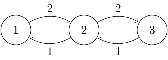
Figure 17.1: Transition diagram for a continuous Markov jump process.

The generator matrix is \[ \mathsf Q = \begin{pmatrix} -2 & 2 & 0 \\ 1 & -3 & 2 \\ 0 & 1 & -1 \end{pmatrix} , \] where the off-diagonal entries are the rates from the diagram, and the diagonal entries are chosen to make sure the rows add up to 0.

The transition matrix of the jump chain is \[ \mathsf R = \begin{pmatrix} 0 & 1 & 0 \\ \frac13 & 0 & \frac23 \\ 0 & 1 & 0 \end{pmatrix} , \] where we set the diagonal elements equal to 0, then normalize each row so that it adds up to 1.

So, for example, starting from state 2, we wait for a holding time $T_1 \sim \operatorname{Exp}(q_2) = \operatorname{Exp}(-q_{22}) = \operatorname{Exp}(3)$. We then move to state 1 with probability $r_{21} = q_{21}/q_2 = \frac13$ and to state 3 with probability $r_{23} = q_{23}/q_2 = \frac23$.

Suppose we move to state 1. Then we stay in state 1 for a time $\operatorname{Exp}(q_1) = \operatorname{Exp}(2)$, before moving with certainty back to state 2. And so on.

Example 17.2 Consider the Markov jump process with state space $\mathcal S = \{A,B,C\}$ and this transition rate diagram.

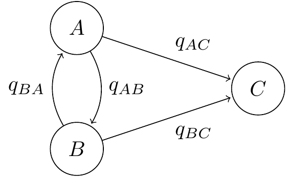
Figure 17.2: Transition diagram for a continuous Markov jump process with an absorbing state.

The generator matrix is \[ \mathsf Q = \begin{pmatrix} -q_A & q_{AB} & q_{AC} \\ q_{BA} & -q_B & q_{BC} \\ 0 & 0 & 0\end{pmatrix} , \] where $q_A = q_{AB} + q_{AC}$ and $q_B = q_{BA} + q_{BC}$. Here, state C is an absorbing state, so if we ever reach it, we stay there forever. So the jump chain has transition rates \[ \mathsf R = \begin{pmatrix} 0 & q_{AB}/q_A & q_{AC}/q_A \\ q_{BA}/q_B & 0 & q_{BC}/q_B \\ 0 & 0 & 1 \end{pmatrix} . \]

Example 17.3 The Poisson process with rate $\lambda$ has state space $\mathcal S = \mathbb Z_+ = \{0,1,2,\dots\}$. The transition rates from $i$ to $i+1$ are $q_{i,i+1} = \lambda$, and all other transition rates are 0. So the generator matrix is \[ \mathsf Q = \begin{pmatrix} -\lambda & \lambda & 0 & 0 & \\ 0 & -\lambda & \lambda & 0 & \\ 0 & 0 & -\lambda & \lambda & \\ & & & \ddots & \ddots \\ \end{pmatrix}. \] The jump chain is very boring: it starts from 0 and moves with certainty to 1, then with certainty to 2, then to 3, and so on.

17.3 A brief note on explosion

There is one point we have to be a little careful about with when dealing with continuous time processes with an infinite state space – the potential of “explosion”. Explosion is when the process can get arbitrarily large in finite time. Think, for example, of a birth process with birth rates $\lambda_j = \lambda j^2$. The $n$th birth is expected to be occur at time \[ \sum_{j=1}^n \frac{1}{\lambda_j} = \frac{1}{\lambda} \sum_{j=1}^n \frac{1}{n^2} . \] But this has a finite limit as $n \to \infty$, meaning we expect to get infinitely many births in a finite amount of time.

When explosion happens, it can then be rather difficult to define what’s going on. In that birth process, for example, the state space is $\mathcal S = \mathbb Z_+$; but after some finite time, we have $X(t) > j$ for all $j \in \mathcal S$ – so what state is the process in?

Although there are often technical fixes that can get around this problem (doing things like creating an “infinity” state, or restarting the process from $X(0)$ again), we will not concern ourselves with them here. We shall normally deal with finite state spaces, where explosion is not a concern. When we do use infinite state space models (such as birth processes, for example), we shall only look at examples that explode with probability 0.

In the next section, we look at how to find the transition probilities $p_{ij}(t) = \mathbb P(X(t) = j \mid X(0) = i)$, which are the equivalents to the $n$-step transition probabilities in discrete time.