Section 6 Examples from actuarial science

Three Markov chain models for insurance problems

In this lecture we’ll set up three simple models for an insurance company that can be analysed using ideas about Markov chains. The first example has a direct Markov chain model. For the second and third examples, we will have to be clever to find a Markov chain associated to the situation.

6.1 A simple no-claims discount model

A motor insurance company puts policy holders into three categories:

no discount on premiums (state 1)
25% discount on premiums (state 2)
50% discount on premiums (state 3)

New policy holders start with no discount (state 1). Following a year with no insurance claims, policy holders move up one level of discount. If they start the year in state 3 and make no claim, they remain in state 3. Following a year with at least one claim, they move down one level of discount. If they start the year in state 1 and make at least one claim, they remain in state 1. The insurance company believes that probability that a motorist has a claim free year is $\frac34$.

We can model this directly as a Markov chain:

the state space $\mathcal S = \{1,2,3\}$ is discrete;
the time index is discrete, as we have one discount level each year;
the probability of being in a certain state at a future time is completely determined by the present state (the Markov property);
the one-step transition probabilities are not time dependent (time homogeneous).

The transition probability and transition diagram of the Markov chain are: \[ \mathsf P = \begin{pmatrix} \frac14 & \frac34 & 0 \\ \frac14 & 0 & \frac34 \\ 0 & \frac14 & \frac34 \end{pmatrix} . \]

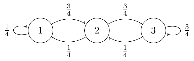
Figure 6.1: Transition diagram for the simple no-claims discount model

Example 6.1 What is the probability of having a 50% reduction to your premium three years from now, given that you currently have no reduction on the premium?

We want to find the three-step transition probability \[ p_{13}(3) = \mathbb P(X_{3} = 3 \mid X_0=1) . \] We can find this by summing over all paths $1 \to k_1 \to k_2 \to 3$. There are two such paths, $1 \to 1 \to 2 \to 3$ and $1 \to 2 \to 3 \to 3$. Thus \[ p_{13}(3) = p_{11}p_{12}p_{23} + p_{12}p_{23}p_{33} = \frac14 \cdot\frac34 \cdot\frac34 + \frac34 \cdot\frac34 \cdot\frac34 = \frac{36}{64} = \frac{9}{16} . \]

Alternatively, we could directly calculate all the three-step transition probabilities by the matrix method, to get \[ \mathsf P(3) = \mathsf P^3 = \mathsf{PPP} = \frac{1}{64} \begin{pmatrix} 7 & 21 & 36 \\ 7 & 12 & 45 \\ 4 & 15 & 45 \end{pmatrix} .\] (You can check this yourself, if you want.) The desired $p_{13}(3)$ is the top right entry $36/64 = 9/16$.

6.2 An accident model with memory

Sometimes, we are presented with a situation where the “obvious” stochastic process is not a Markov chain. But sometimes we can find a related process that is a Markov chain, and study that instead. As an example of this, we consider at a different accident model.

According to a different model, a motorist’s $n$th year of driving is either accident free, or has exactly one accident. (The model does not allow for more than one accident in a year.) Let $Y_n$ be a random variable so that, \[ Y_n=\begin{cases} 0&\text{ if the motorist has no accident in year $n$,}\\ 1&\text{ if the motorist has one accident in year $n$.} \end{cases} \] This defines a stochastic process $(Y_n)$ with finite state space $\mathcal{S}=\{0,1\}$ and discrete time $n = 1,2,3,\dots$.

The probability of an accident in year $n+1$ is modelled as a function of the total number of previous accidents over a function of the number of years in the policy; that is, \[ \mathbb P(Y_{n+1}= 1 \mid Y_n=y_{n},\dots ,Y_2=y_{2},Y_1=y_{1} )=\frac{f(y_1+y_2+\cdots +y_n)}{g(n)}, \] and $Y_{n+1} = 0$ otherwise, where $f$ and $g$ are non-negative increasing functions with $0\leq f(m)\leq g(m)$ for all $m$. (We’ll come back to these conditions in a moment.)

Unfortunately $(Y_n)$ is not a Markov chain – it’s clear that $Y_{n+1}$ depends not only on $Y_n$, the number accidents this year, but the entire history $Y_1, Y_2, \dots, Y_n$.

However, we have a cunning work-around. Define $X_n=\sum_{i=1}^n Y_i$ to be the total number of accidents up to year $n$. Then $(X_n)$ is a Markov chain. In fact, we have \[\begin{align*} \mathbb P(X_{n+1}={}&{}x_{n}+1\mid X_n=x_n, \dots, X_2=x_2, X_1=x_1)\\ &=\mathbb P(Y_{n+1}=1\mid Y_n=x_n - x_{n-1}, \dots Y_2=x_2-x_1, Y_1=x_1)\\ &=\frac{f\big((x_n-x_{n-1}) +\cdots +(x_2-x_1) + x_1\big)}{g(n)}\\ &=\frac{f(x_n)}{g(n)}, \end{align*}\] and $X_{n+1} = x_n$ otherwise. This clearly depends only on $x_n$. Thus we can use Markov chain techniques on $(X_n)$ to lean about the non-Markov process $(Y_n)$.

Note that the probability that $X_{n+1} = x_n$ or $x_n+ 1$ depends not only on $x_n$ but also on the time $n$. So this is a rare example of a time inhomogeneous Markov process, where the transition probabilities do depend on the time $n$.

Before we move on, let’s think about the conditions we placed on this model. First, the condition that $f$ is increasing means that between drivers who have been driving the same number of years, we think the more accident-prone in the past is more likely to have an accident in the future. Second, the condition that $g$ is increasing means that between drivers who have had the same number of accidents, we think the one who has spread those accidents over a longer period of time is less likely to have accidents in the future. Third, the transition probabilities should lie in the range $[0,1]$; but since $\sum_{i=1}^m y_i\leq m$, our condition $0\leq f(m)\leq g(m)$ guaranteed that this is the case.

6.3 A no-claims discount model with memory

Sometimes, we are presented with a stochastic process which is not a Markov chain, but where by altering the state space $\mathcal{S}$ we can end up with a process which is a Markov chain. As such, when making a model, it is important to think carefully about choice of state space. To see this we will return to the no-claims discount example.

Suppose now we have an model with four levels of discount:

no discount (state 1)
20% discount (state 2)
40% discount (state 3)
60% discount (state 4)

If a year is accident free, then the discount increases one level, to a maximum of 60%. This time, if the year has an accident, then the discount decreases by one level if the year previous to that was accident free, but decreases by two levels if the previous year had an accident as well, both to a minimum of no discount.

As before, the insurance company believes that probability that a motorist has a claim-free year is $\frac34 = 0.75$.

We might consider the most natural choice of a state space, where the states are discount levels; say, $\mathcal{S}=\{1,2,3,4\}$. But this is not a Markov chain, since if a policy holder has an accident, we may need to know about the past in order to determine probabilities for future states, which violates the Markov property. In particular, if a motorist is in state 3 (40% discount) and has an accident, they will either move down to level 2 (if they had not crashed the previous year, so had previously been in state 2) or to level 1 (if they had crashed the previous year, so had previously been in state 4) – but that depends on their previous level too, which the Markov property doesn’t allow. (You can check this is the only violation of the Markov property.)

However, we can be clever again, this time in the choice of our state space. Instead, we can split the 40% level into two different states: state “3a” if there was no accident the previous year, and state “3b” if there was an accident the previous year. Our states are now:

no discount (state 1)
20% discount (state 2)
40% discount, no claim in previous year (state 3a)
40% discount, claim in previous year (state 3b)
60% discount (state 4)

Now this is a Markov chain, because the new states 3s carry with them the memory of the previous year, to ensure the Markov property is preserved. Under the assumption of 25% of drivers having an accident each year, the transition matrix is \[ \mathsf P=\begin{pmatrix} 0.25 & 0.75 & 0 & 0 & 0\\ 0.25 & 0 & 0.75 & 0 & 0\\ 0 & 0.25 & 0 & 0 & 0.75\\ 0.25 & 0 & 0 & 0 & 0.75\\ 0 & 0 & 0 & 0.25 & 0.75\end{pmatrix}. \] The transition diagram is shown below. (Recall that we don’t draw arrows with probability 0.)

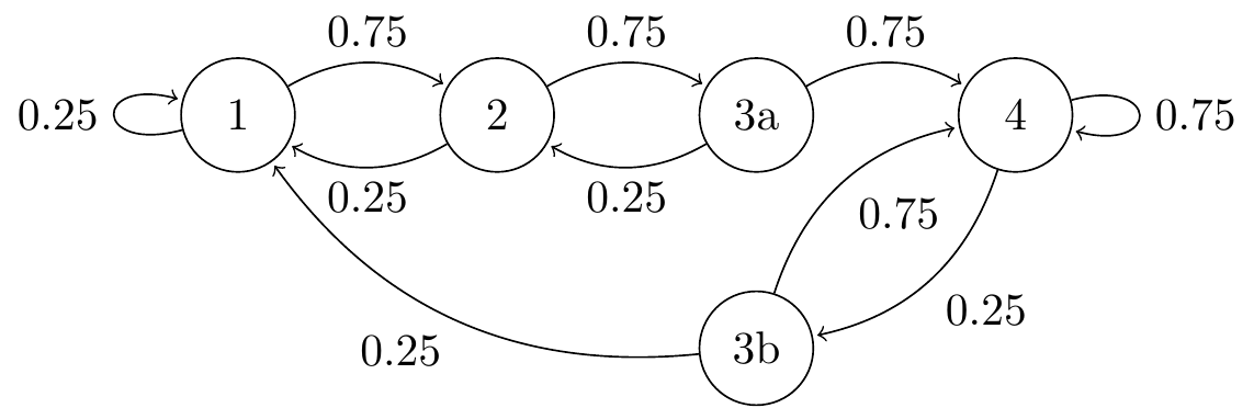
Figure 6.2: Transition diagram for the no-claims discount model with memory

Note that when we move up from state 2, we go to 3a (no accident in the previous year); but when we move down from state 4, we go to 3b (accident in the previous year).

In the next section, we look at how to study big Markov chains by splitting them into smaller pieces called “classes”.