Section 21 Queues

The M/M/$\infty$ infinite server process
The M/M/1 single server queue

21.1 M/M/∞ infinite server process

In a mathematical model for a queue, individuals arrive, receive a service, and leave. In our first example, individuals receive service as soon as they arrive – so there is no actual “queueing”. In our second example, later, individuals will actually queue up and wait until the server is able to serve them.

Our first process as follows. Individuals arrive like a Poisson process of rate $\lambda$. Then they receive a service which takes time $\operatorname{Exp}(\mu)$, independent of everything else, and then they leave.

This can be a useful model for many applications: for example, visitors watching a livestream on a website could arrive at the website like a Poisson process of rate $\lambda$ and watch the livestream for a $\operatorname{Exp}(\mu)$ amount of time. Other models could include the number of students in the University library, the number of insurance contracts held by an insurance broker, or the number of files being downloaded from a server.

The number of individuals $(X(t))$ in the process (that is, receiving the service) at time $t$ is a Markov jump process with arrival rates $q_{i,i+1} = \lambda$. The rate of departures when $i$ individuals are being serviced has the rate and $q_{i,i-1} = i\mu$, because, thanks to the memoryless property of the exponential distribution, the first service time to finish is the minimum of $i$ remaining exponential service times, and this is exponential with rate $i\mu$. Since rows of a generator matrix sum to 0, we have $q_i = -q_{ii} = \lambda + i\mu$.

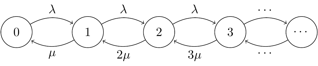
Figure 21.1: An M/M/∞ queue

Writing $\mathsf Q = (q_{ij})$ as a matrix, it is \[ \mathsf Q = \begin{pmatrix} -\lambda & \lambda & & & & \\ \mu & -(\lambda + \mu) & \lambda & & & \\ & 2\mu & -(\lambda + 2\mu) & \lambda & & \\ & & 3\mu & -(\lambda + 3\mu) & \lambda & \\ & & & \ddots & \ddots & \ddots \end{pmatrix} , \] where all the blank entries are 0.

This process is called the M/M/$\infty$ process.

The first M stands for memoryless arrivals, which means the arrivals process is a Poisson process, which has exponential – and therefore memoryless – interarrival times.
The second M stands for memoryless service times, which means the service times are exponentially distributed, and hence have the memoryless property.
The $\infty$ stands for infinite servers, which means there is no limit on how many individuals can be serviced at once.

Two questions we might want to know the answer to are these:

In the long run, what’s the average number of individuals being serviced?
In the long run, for what proportion of the time are all the servers idle?

To find out about this long run behaviour, we need to calculate the stationary distribution. The stationary distribution solves $\boldsymbol\pi\mathsf Q = \mathsf 0$. Thus we have \[\begin{equation} \lambda \pi_{i-1} - (\lambda + i\mu)\pi_i + (i+1)\mu \pi_{i+1} = 0 \tag{21.1} \end{equation}\] for $i \geq 1$, and \[\begin{equation} -\lambda \pi_0 + \mu \pi_1 = 0 \tag{21.2} \end{equation}\] from the first column of $\mathsf Q$.

Rearranging (21.2) gives $\pi_1 = \rho \pi_0$, where $\rho = \lambda/\mu$. Putting this into (21.1) for $i = 1$ gives (after some algebra) $\pi_2 = \pi_0 \rho^2 / 2$. Putting that into for $i = 2$ gives $\pi_3 = \pi_0 \rho^3 / 6$.vThis looks suspiciously like the stationary distribution might be the Poisson distribution with rate $\rho$; that is, $\pi_i = \pi_0 \rho^i / i! = \mathrm{e}^{-\rho} \rho^i / i!$.

Theorem 21.1 Let $(X(t))$ be an M/M/$\infty$ process with arrivals at rate $\lambda$ and service at rate $\mu$. The process has the stationary distribution $\pi_i = \mathrm{e}^{-\rho} \rho^i / i!$, corresponding to $X(t) \sim \mathrm{Po}(\rho)$, where $\rho = \lambda/\mu$.

Proof. We know that this $\boldsymbol\pi$ is a distribution. We must check that $\boldsymbol\pi$ fulfills $\boldsymbol\pi \mathsf Q = \mathbf 0$. We’ve already checked (21.2). For $i \geq 1$, we have from (21.1), \[\begin{align*} \lambda \pi_{i-1}{} - {}&(\lambda + i\mu)\pi_i + (i+1)\mu \pi_{i+1} \\ &= \lambda\, \mathrm{e}^{-\rho} \frac{\rho^{i-1}}{(i-1)!} - (\lambda + i\mu) \,\mathrm{e}^{-\rho} \,\frac{\rho^i}{i!} + (i+1)\mu \,\mathrm{e}^{-\rho} \frac{\rho^{i+1}}{(i+1)!} \\ &= \lambda \mathrm{e}^{-\rho} \frac{i}{\rho} \frac{\rho^i}{i!} - (\lambda + i\mu) \,\mathrm{e}^{-\rho} \,\frac{\rho^i}{i!} + \mu \mathrm{e}^{-\rho} \rho \,\frac{\rho^i}{i!} \\ &= \mathrm{e}^{-\rho} i\mu \frac{\rho^i}{i!} - (\lambda + i\mu) \,\mathrm{e}^{-\rho} \,\frac{\rho^i}{i!} + \mathrm{e}^{-\rho} \lambda \,\frac{\rho^i}{i!}\\ &= \mathrm{e}^{-\rho} \,\frac{\rho^i}{i!} \big( i \mu - (\lambda + i \mu) + \lambda \big) \\ &= 0 , \end{align*}\] as desired.

This process is clearly irreducible, and since it has a stationary distribution it must be positive recurrent. So, by the limit theorem, we see that $\boldsymbol\pi$ is also the equilibrium distribution. By the ergodic theorem, the long-run amount of time spent in each state is governed by $\boldsymbol\pi$.

In answer to question 1, the average number of individuals being serviced is $\mathbb E (\text{Po}(\rho)) = \rho = \lambda/\mu$. In answer to question 2, the long-run proportion of time the process is empty is $\pi_0 = \mathrm{e}^{-\rho} = \mathrm{e}^{-\lambda/\mu}$.

21.2 M/M/1 single server queue

We now consider a slightly different process with only one server. This is called an M/M/1 queue, where the “1” is the number of servers.

As before, individuals arrive as a Poisson process of rate $\lambda$. If there is no one currently being serviced, the individual goes straight to the server, and begins an $\operatorname{Exp}(\mu)$ service time. Otherwise, they have to join a queue waiting for the server to become free. When the server finishes serving one individual, then, provided the queue is nonempty, they immediately begin to service the individual who has been waiting in the queue for the longest time.

This is again a very useful model for many applications. For example, it could model a lecturer’s office hours: students arrive at my office at rate $\lambda$; if I’m free, I can immediately answer their question, which will take an $\text{Exp}(\mu)$ amount of time; but if I’m already dealing with a student, they must join a queue and wait until I am free. This could also model purchases at a shop with a single till, phone calls to a receptionist, or the work of a self-employed person on different tasks.

Let $(X(t))$ be the number of individuals in the process at time $t$. That could be $X(t) = 0$, if the server is free; $X(t) = 1$ if one individual is currently being serviced but no one else is waiting; or $X(t) = x > 1$ if one individual is being services and $x - 1$ individuals are waiting in the queue.. Individuals enter the queue at rate $q_{i,i+1} = \lambda$. When $i \geq 1$, meaning someone is being serviced, we have departures at rate $q_{i,i-1} = \mu$. Thus $q_i = -q_{ii} = \lambda + \mu$ for $i \geq 1$, and $q_0 = -q_{00} = \lambda$.

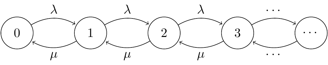
Figure 21.2: An M/M/1 queue

The matrix $\mathsf Q$ this time is \[ \mathsf Q = \begin{pmatrix} -\lambda & \lambda & & & & \\ \mu & -(\lambda + \mu) & \lambda & & & \\ & \mu & -(\lambda + \mu) & \lambda & & \\ & & \mu & -(\lambda + \mu) & \lambda & \\ & & & \ddots & \ddots & \ddots \end{pmatrix} . \]

The first thing we would like to know is if the queue keeps getting longer and longer, or whether eventually every individual is serviced.

For this continuous time jump process $(X(t))$, the discrete time jump chain $(Y_n)$ is a simple random walk with up probability $p = \lambda/(\lambda + \mu)$, down probability $q = \mu/(\lambda + \mu)$, and a reflecting barrier at 0. Recall that this Markov chain is transient for $p > q$, null recurrent for $p = q$, and positive recurrent for $p < q$. Thus we see that:

For $\lambda > \mu$, the queue is transient, and eventually the length of the queue will grow longer and longer and never clear. This is clearly highly undesirable.
For $\lambda = \mu$, the queue is null recurrent, so while the queue will eventually clear, the expected time for it to do so is infinite, so the queue will get very long, and individuals will may have to wait for an extremely long time. This is also undesirable.
For $\lambda < \mu$, the queue is positive recurrent, so while individuals may sometimes have to wait, the queue will clear fairly regularly. This is what we want.

In what follows, we consider only the “good” case $\lambda < \mu$. Again we have two questions:

In the long run, what’s the average number of individuals being serviced?
In the long run, for what proportion of the time is the server idle and for what proportion of time is the server busy?

Again, we look for a stationary distribution, which will tell us about the long term behaviour of the queue. The equation $\boldsymbol\pi\mathsf Q = \mathbf 0$ this time becomes \[ \mu \pi_{i+1} - (\lambda + \mu) \pi_i + \lambda \pi_{i-1} = 0 \qquad \text{for $i \geq 1$} , \] together with the initial condition $\mu \pi_1 - \lambda \pi_0 = 0$ from the first column of $\mathsf Q$, and the normalising condition $\sum_i \pi_i = 1$.

We recognise this as a linear difference equation. The characteristic equation (using $\alpha$ where we used $\lambda$ previously, since $\lambda$ is already in use) is \[ \mu \alpha^2 - (\lambda + \mu)\alpha + \lambda = (\alpha - 1)(\mu \alpha - \lambda ) = 0 . \] This has solutions $\alpha = 1$ and $\alpha = \rho$, where $\rho = \lambda/\mu < 1$, so the general solution to the equation is $\pi_i = A + B\rho^i$.

The initial condition gives \[ \mu \pi_1 - \lambda \pi_0 = \mu(A + B\rho) - \lambda(A + B) = A\mu + B\lambda - A \lambda - B\lambda = A(\mu - \lambda) = 0 . \] Since $\lambda < \mu$, we must have $A = 0$. The normalising condition requires \[ \sum_{i=0}^\infty \pi_i = \sum_{i=0}^\infty B\rho^i = \frac{B}{1- \rho} = 1 , \] where we’ve used the formula for the sum of a geometric progression with $\rho < 1$, which gives $B = 1 - \rho.$

Thus we have the stationary distribution $\pi_i = (1 - \rho)\rho^i$, which is a geometric distribution (the version that starts from $i = 0$).

Theorem 21.2 Let $(X(t))$ be an M/M/1 queue with arrivals at rate $\lambda$ and service at rate $\mu > \lambda$. The queue has the stationary distribution $\pi_i = (1 - \rho)\rho^i$, corresponding to $X(t) \sim \mathrm{Geom}(\rho)$, where $\rho = \lambda/\mu < 1$.

By the limit theorem, this is an equilibrium distribution, and the ergoic theorem also applied.

To answer question 1, the long-run average number of individuals in the process will be \[ \mathbb E\big(\text{Geom}(\rho)\big) = \frac{\rho}{1-\rho} = \frac{\lambda}{\mu - \lambda} . \] If $\lambda$ is only slightly smaller than $\mu$ then this number can be quite large; in this case the queue can get very long, even though we know it will clear in a reasonable finite-expectation time. To answer question 2, the server will be free a proportion $\pi_0 = 1 - \rho = 1 - \lambda/\mu$ of the time and busy a proportion $1 - \pi_0 = \lambda/\mu$ of the time, in the long run. Again, if $\lambda$ is only slightly smaller than $\mu$, then the server will be busy most of the time.

This brings us to the end of the mathematical material in this module. In the next section, we summarise Part II on continuous time Markov jump processes and discuss the forthcoming exam.