Section 5 Discrete time Markov chains

Definition of time homogeneous discrete time Markov chains
Calculating $n$-step transition properties
The Chapman–Kolomogorov equations

5.1 Time homogeneous discrete time Markov chains

So far we’ve seen a a few examples of stochastic processes in discrete time and discrete space with the Markov memoryless property. Now we will develop the theory more generally.

To define a so-called “Markov chain”, we first need to say where we start from, and second what the probabilities of transitions from one state to another are.

In our examples of the simple random walk and gambler’s ruin, we specified the start point $X_0 = i$ exactly, but we could pick the start point at random according to some distribution $\lambda_i = \mathbb P(X_0 = i)$.

After that, we want to know the transition probabilities $\mathbb P(X_{n+1} = j \mid X_n = i)$ for $i,j \in \mathcal S$. Here, because of the Markov property, the transition probability only needs to condition on the state we’re in now $X_n = i$, and not on the whole history of the process.

In the case of the simple random walk, for example, we had initial distribution \[ \lambda_i = \mathbb P(X_0 = i) = \begin{cases} 1 & \text{if $i = 0$} \\ 0 & \text{otherwise} \end{cases} \] and transition probabilities \[ \mathbb P(X_{n+1} = j \mid X_n = i) = \begin{cases} p & \text{if $j = i+1$} \\ q & \text{if $j = i-1$} \\ 0 & \text{otherwise.} \end{cases} \]

For the random walk (and also the gambler’s ruin), the transition probabilities $\mathbb P(X_{n+1} = j \mid X_n = i)$ don’t depend on $n$; in other words, the transition probabilities stay the same over time. A Markov process with this property is called time homogeneous. We will always consider time homogeneous processes from now on (unless we say otherwise).

Let’s write $p_{ij} = \mathbb P(X_{n+1} = j \mid X_n = i)$ for the transition probabilities, which are independent of $n$. We must have $p_{ij} \geq 0$, since it is a probability, and we must also have $\sum_j p_{ij} = 1$ for all states $i$, as this is the sum of the probabilities of all the places you can move to from state i.

Definition 5.1 Let $(\lambda_i)$ be a probability distribution on a sample space $\mathcal S$. Let $p_{ij}$, where $i,j \in \mathcal S$, be such that $p_{ij} \geq 0$ for all $i,j$, and $\sum_j p_{ij} = 1$ for all $i$. Let the time index be $n = 0,1,2,\dots$. Then the time homogeneous discrete time Markov process or Markov chain $(X_n)$ with initial distribution $(\lambda_i)$ and transition probabilities $(p_{ij})$ is defined by \[\begin{gather*} \mathbb P(X_0 = i) = \lambda_i ,\\ \mathbb P(X_{n+1} = j \mid X_n = i, X_{n-1} = x_{n-1}, \dots, X_0 = x_0) = \mathbb P(X_{n+1} = j \mid X_n = i) = p_{ij} . \end{gather*}\]

When the state space is finite (and even sometimes when it’s not), it’s convenient to write the transition probabilities $(p_{ij})$ as a matrix $\mathsf P$, called the transition matrix, whose $(i,j)$th entry is $p_{ij}$. Then the condition that $\sum_j p_{ij} = 1$ is the condition that each of the rows of $\mathsf P$ add up to $1$.

Example 5.1 In this notation, what is $\mathbb P(X_0 = i \text{ and } X_1 = j)$?

First we must start from $i$, and then we must move from $i$ to $j$, so \[ \mathbb P(X_0 = i \text{ and } X_1 = j) = \mathbb P(X_0 = i)\mathbb P(X_1 = j \mid X_0 = i) = \lambda_i p_{ij} . \]

In this notation, what is $\mathbb P(X_{n+2} = j \text{ and } X_{n+1} = k \mid X_n = i)$?

First we must move from $i$ to $k$, then we must move from $k$ to $j$, so \[\begin{align*} \mathbb P(X_{n+2} = j \text{ and } X_{n+1} = k \mid X_n = i) &= \mathbb P(X_{n+1} = k \mid X_n = i)\mathbb P(X_{n+2} = j \mid X_{n+1} = k) \\ &= p_{ik}p_{kj} . \end{align*}\] Note that the term $\mathbb P(X_{n+2} = j \mid X_{n+1} = k)$ did not have to depend on $X_n$, thanks to the Markov property.

5.2 A two-state example

Consider a simple two-state Markov chain with state space $\mathcal S = \{0,1\}$ and transition matrix \[ \mathsf P = \begin{pmatrix} p_{00} & p_{01} \\ p_{10} & p_{11} \end{pmatrix} = \begin{pmatrix} 1-\alpha & \alpha \\ \beta & 1-\beta \end{pmatrix} \] for some $0 < \alpha, \beta < 1$. Note that the rows of $\mathsf P$ add up to $1$, as they must.

We can illustrate $\mathsf P$ by a transition diagram, where the blobs are the states and the arrows give the transition probabilities. (We don’t draw the arrow if $p_{ij} = 0$.) In this case, our transition diagram looks like this:

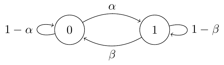
Figure 5.1: Transition diagram for the two-state Markov chain

We can use this as a simple model of a broken printer, for example. If the printer is broken (state 0) on one day, then with probability $\alpha$ it will be fixed (state 1) by the next day; while if it is working (state 1), then with probability $\beta$ it will have broken down (state 0) by the next day.

Example 5.2 If the printer is working on Monday, what’s the probability that it also is working on Wednesday?

If we call Monday day $n$, then Wednesday is day $n+2$, and we want to find the two-step transition probability. \[ p_{11}(2) = \mathbb P (X_{n+2} = 1 \mid X_n = 1) . \] The key to calculating this is to condition on the first step again – that is, on whether the printer is working on Tuesday. We have \[\begin{align*} p_{11}(2) &= \mathbb P (X_{n+1} = 0 \mid X_n = 1)\,\mathbb P (X_{n+2} = 1 \mid X_{n+1} = 0, X_n = 1) \\ &\qquad{} + \mathbb P (X_{n+1} = 1 \mid X_n = 1)\,\mathbb P (X_{n+2} = 1 \mid X_{n+1} = 1, X_n = 1) \\ &= \mathbb P (X_{n+1} = 0 \mid X_n = 1)\,\mathbb P (X_{n+2} = 1 \mid X_{n+1} = 0) \\ &\qquad{} + \mathbb P (X_{n+1} = 1 \mid X_n = 1)\,\mathbb P (X_{n+2} = 1 \mid X_{n+1} = 1) \\ &= p_{10}p_{01} + p_{11}p_{11} \\ &= \beta\alpha + (1-\beta)^2 . \end{align*}\] In the second equality, we used the Markov property to mean conditional probabilities like $\mathbb P(X_{n+2} = 1 \mid X_{n+1} = k)$ did not have to depend on $X_n$.

Another way to think of this as we summing the probabilities of all length-2 paths from 1 to 1, which are $1\to 0\to 1$ with probability $\beta\alpha$ and $1 \to 1 \to 1$ with probability $(1-\beta)^2$

5.3 n-step transition probabilities

In the above example, we calculated a two-step transition probability $p_{ij}(2) = \mathbb P (X_{n+2} = j \mid X_n = i)$ by conditioning on the first step. That is, by considering all the possible intermediate steps $k$, we have \[ p_{ij}(2) = \sum_{k\in\mathcal S} \mathbb P (X_{n+1} = k \mid X_n = i)\mathbb P (X_{n+2} = j \mid X_{n+1} = k) = \sum_{k\in\mathcal S} p_{ik}p_{kj} . \]

But this is exactly the formula for multiplying the matrix $\mathsf P$ with itself! In other words, $p_{ij}(2) = \sum_{k} p_{ik}p_{kj}$ is the $(i,j)$th entry of the matrix square $\mathsf P^2 = \mathsf{PP}$. If we write $\mathsf P(2) = (p_{ij}(2))$ for the matrix of two-step transition probabilities, we have $\mathsf P(2) = \mathsf P^2$.

More generally, we see that this rule holds over multiple steps, provided we sum over all the possible paths $i\to k_1 \to k_2 \to \cdots \to k_{n-1} \to j$ of length $n$ from $i$ to $j$.

Theorem 5.1 Let $(X_n)$ be a Markov chain with state space $\mathcal S$ and transition matrix $\mathsf P = (p_{ij})$. For $i,j \in \mathcal S$, write \[ p_{ij}(n) = \mathbb P(X_n = j \mid X_0 = i) \] for the $n$-step transition probability. Then \[ p_{ij}(n) = \sum_{k_1, k_2, \dots, k_{n-1} \in \mathcal S} p_{ik_1} p_{k_1k_2} \cdots p_{k_{n-2}k_{n-1}} p_{k_{n-1}j} . \] In particular, $p_{ij}(n)$ is the $(i,j)$th element of the matrix power $\mathsf P^n$, and the matrix of $n$-step transition probabilities is given by $\mathsf P(n) = \mathsf P^n$.

The so-called Chapman–Kolmogorov equations follow immediately from this.

Theorem 5.2 (Chapman–Kolmogorov equations) Let $(X_n)$ be a Markov chain with state space $\mathcal S$ and transition matrix $\mathsf P = (p_{ij})$. Then, for non-negative integers $n,m$, we have \[ p_{ij}(n+m) = \sum_{k \in \mathcal S} p_{ik}(n)p_{kj}(m) , \] or, in matrix notation, $\mathsf P(n+m) = \mathsf P(n)\mathsf P(m)$.

In other words, a trip of length $n + m$ from $i$ to $j$ is a trip of length $n$ from $i$ to some other state $k$, then a trip of length $m$ from $k$ back to $j$, and this intermediate stop $k$ can be any state, so we have to sum the probabilities.

Of course, once we know that $\mathsf P(n) = \mathsf P^n$ is given by the matrix power, it’s clear to see that $\mathsf P(n+m) = \mathsf P^{n+m} = \mathsf P^n \mathsf P^m = \mathsf P(n)\mathsf P(m)$.

Sidney Chapman (1888–1970) was a British applied mathematician and physicist, who studied applications of Markov processes. Andrey Nikolaevich Kolmogorov (1903–1987) was a Russian mathematician who did very important work in many different areas of mathematics, is considered the “father of modern probability theory”, and studied the theory of Markov processes. (Kolmogorov is also my academic great-great-grandfather.)

Example 5.3 In our two-state broken printer example above, the matrix of two-state transition probabilities is given by \[\begin{align*} \mathsf P(2) = \mathsf P^2 &= \begin{pmatrix} 1-\alpha & \alpha \\ \beta & 1-\beta \end{pmatrix} \begin{pmatrix} 1-\alpha & \alpha \\ \beta & 1-\beta \end{pmatrix} \\ &= \begin{pmatrix} (1-\alpha)^2 + \alpha\beta & (1-\alpha)\alpha + \alpha(1-\beta) \\ \beta(1-\alpha) + (1-\beta)\beta & \beta\alpha + (1-\beta)^2 \end{pmatrix} , \end{align*}\] where the bottom right entry $p_{11}(2)$ is what we calculated earlier.

One final comment. It’s also convenient to consider the initial distribution $\boldsymbol\lambda = (\lambda_i)$ as a row vector. The first-step distribution is given by \[ \mathbb P(X_1 = j) = \sum_{i \in \mathcal S} \lambda_i p_{ij} , \] by conditioning on the start point. This is exactly the $j$th element of the vector–matrix multiplication $\boldsymbol\lambda \mathsf P$. More generally, the row vector of of probabilities after $n$ steps is given by $\boldsymbol\lambda \mathsf P^n$.

In the next section, we look at how to model some actuarial problems using Markov chains.