Section 19 Class structure and hitting times

Communicating classes
Hitting probabilities and expected hitting times
Recurrence and transience

When we studied discrete time Markov chains, we considered matters including communicating classes, periodicity, hitting probabilities and expected hitting times, recurrence and transience, stationary distributions, convergence to equilibrium, and the ergodic theorem. In this section and the next, we develop this theory for continuous time Markov jump processes. Luckily, things will be simpler this time round, as we will often be able to use exactly the same techniques as the discrete time case, often by looking at the discrete time jump chain.

19.1 Communicating classes

In discrete time, we said that $j$ is accessible from $i$, and wrote $i \to j$ if $p_{ij}(n) > 0$ for some $n$. This allowed us to split the state space into communicating classes. We can do exactly the same in discrete time.

Definition 19.1 Let $(X(t))$ be a Markov jump process on a state space $\mathcal S$ with transition semigroup $(\mathsf P(t))$. We say that a state $j \in \mathcal S$ is accessible from another state $i \in \mathcal S$, and write $i \to j$ if $p_{ij}(t) > 0$ for some $t \geq 0$. If $i \to j$ and $j \to i$, we say that $i$ communicates with $j$ and write $i \leftrightarrow j$.

The equivalence relation $\leftrightarrow$ partitions $\mathcal S$ into equivalence classes, which we call communicating classes.

If all states are in the same class, the jump process is irreducible. A class $C$ is closed if $i \to j$ for $i \in C$ means that $j \in C$ also. If $i$ is a closed class $\{i\}$ be itself, then $i$ is an absorbing state.

Recall that each state $i$ is in exactly one communicating class, and that communicating class is the set of all $j$ such that $i \leftrightarrow j$.

If $p_{ij}(t) > 0$, then this means there is some sequence of jumps that can take us from $i$ to $j$. This means that, letting $\mathsf R = (r_{ij})$ be the transition matrix for the jump chain $(Y_n)$, we have that $p_{ij}(t) > 0$ for some $t$ if and only if $r_{ij}(n) > 0$ for some $n$. So the communicating classes for a Markov jump process are exactly the same as the communicating classes in its discrete time jump chain.

Further, since $r_{ij} > 0$ if and only if $q_{ij} > 0$, we can tell what the communicating classes are directly from the transition rate diagram.

Example 19.1 Write down the communicating classes for the Markov jump process with generator matrix \[ \mathsf Q = \begin{pmatrix} -2 & 2 & 0 \\ 1 & -3 & 2 \\ 0 & 0 & 0 \end{pmatrix}. \]

The transition rate diagram is

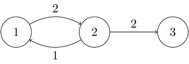
Figure 19.1: A Markov jump process with three states and two communicating classes.

We immediately see that the communicating classes are $\{1,2\}$, which is not closed, and $\{3\}$ which is closed, so 3 is an absorbing state. The process is not irreducible.

19.2 A brief note on periodicity

In discrete time we had to worry about periodic behaviour, especially when considering long-term behaviour like the existence of an equilibrium distribution. However, for a continuous time jump process, it’s possible stay in a state for any positive real-number amount of time. Thus (with probability 1) we never see periodic behaviour, and we don’t have to worry about this.

This is one way in which continuous time processes are actually more pleasant to deal with than discrete time processes.

19.3 Hitting probabilities and expected hitting times

Recall that the hitting probability $h_{iA}$ is the probability of reaching some state $j \in A$ at any point in the future starting from $i$, and the expected hitting time $\eta_{iA}$ is the expected amount of time to get there. We found these in discrete time by forming simultaneous equations by conditioning on the first step.

For hitting probabilities, we just care about where we jump to, and not how long we wait. Thus we are free to consider only the jump chain $(Y_n)$ and its transition matrix $\mathsf R$. Everything works exactly as in discrete time.

Example 19.2 Continuing with the previous example, calculate $h_{21}$, the probability of hitting state 1 starting from 2.

The jump chain has transition matrix \[ \mathsf R = \begin{pmatrix} 0 & 1 & 0 \\[0.3ex] \tfrac13 & 0 & \tfrac23 \\[0.3ex] 0 & 0 & 1 \end{pmatrix} . \]

By conditioning on the first step, we have \[ h_{21} = \tfrac13 h_{11} + \tfrac23 h_{31} = \tfrac13 \times 1 + \tfrac23 \times 0 = \tfrac13 , \] where $h_{31} = 0$ since 3 is an absorbing state. Hence, $h_{21} = \frac13$.

For expected hitting times, we have to more careful, as we will spend a random amount of time in the current state before moving on. In particular, the time we spend in state $i$ is exponential with rate $q_i = -q_{ii}$, so has expected value $1/q_i$.

We illustrate the approach with an example.

Example 19.3 Continuing with the same example, find the expected hitting time $\eta_{13}$.

We condition on the first step. Starting from 1, we spend an expected time $1/q_1 = \frac12$ in state 1 before moving on with certainty to state 2, so \[ \eta_{13} = \tfrac12 + \eta_{23} . \] From state 2, we have a holding time with expectation $1/q_2 = \frac13$, before moving to 1 with probability $\frac13$ and 2 with probability $\frac23$. So \[ \eta_{23} = \tfrac13 + \tfrac13 \eta_{12} + \tfrac23 \eta_{23} = \tfrac13 + \tfrac13 \eta_{12} , \] since $\eta_{33}$ is of course 0. Substituting the second equation into the first, we get \[ \eta_{13} = \tfrac12 + \tfrac13 + \tfrac13 \eta_{13} , \] which rearranges to $\frac23 \eta_{13} = \frac56$, giving $\eta_{13} = \frac54$.

We have to be a little bit careful with return times and return probabilities. The return time is now the first time we come back to a state after having left it. In particular, if we begin in state $i$, we first leave at time $T_1 \sim \operatorname{Exp}(q_i)$, and we are looking for the first return after that.

So, specifically, the definitions of return time, return probability, and expected return time are \[\begin{gather*} M_i = \min \big\{t > T_1 : X(t) = i \big\} , \\ m_i = \mathbb P\big(X(t) = i \text{ for some $t > T_1$} \mid X(0) = i \big) = \mathbb P \big( M_i < \infty \mid X(0) = i \big) ,\\ \mu_i = \mathbb E\big( M_i \mid X(0) = i \big). \end{gather*}\] In particular, if $q_i = 0$, so $T_1 = \infty$ and we never leave state $i$, the return time, return probability and expected return time are not defined. (We will have no use for them.)

By conditioning on the first step, it’s clear we have \[ m_i = \sum_j r_{ij} h_{ji} = \sum_{j \neq i} \frac{q_{ij}}{q_i} \, h_{ji}, \qquad \mu_i = \frac{1}{q_i} + \sum_j r_{ij} \eta_{ji} = \frac{1}{q_i} \bigg(1 + \sum_{j \neq i} q_{ij} \eta_{ji} \bigg). \]

We see (except for the $q_i = 0$ case) that the return probability is the same in the jump chain as it is in the original Markov jump process, as was the case for the hitting probability, but for the expected return time we have to remember the random amount of time spent in each state.

19.4 Recurrence and transience

In discrete time, we said a state $i$ was recurrent if the return probability $m_i = 1$ equalled 1 and transient if the return probability $m_i < 1$ was strictly less than 1. We take almost the same definition in continuous time – the difference is that if we never leave a state, because $q_i = 0$, we should call state $i$ recurrent.

Definition 19.2 If a state $i \in \mathcal S$ has return probability $m_i = 1$ or has $q_i = 0$, we say that $i$ is recurrent. If $m_i < 1$, we say that $i$ is transient.

Suppose $i$ is recurrent. If the expected return time $\mu_i < \infty$ is finite or $q_i = 0$, we say that $i$ is positive recurrent. If the expected return time $\mu_i = \infty$ is infinite, we say that $i$ is null recurrent.

We see that the return probability is totally determined the jump chain, so whether a state is recurrent or transient can be decided exactly as in the discrete case. In particular, in a communicating class either all states are transient or all states are recurrent. As before, finite closed classes are recurrent, and non-closed classes are transient.

Example 19.4 Picking up our example again, $\{1,2\}$ is not closed, so is transient, while the absorbing state 3 is positive recurrent.

In the next section, we look at the long-term behaviour of continuous time Markov jump processes in a similar way to discrete time Markov chains: stationary distributions, convergence to equilibrium, and an ergodic theorem.